Do-It-Yourself

In this section, we are going to try

import geopandas
import contextily
from pysal.lib import examples

/tmp/ipykernel_9836/2071694180.py:1: UserWarning: Shapely 2.0 is installed, but because PyGEOS is also installed, GeoPandas will still use PyGEOS by default for now. To force to use and test Shapely 2.0, you have to set the environment variable USE_PYGEOS=0. You can do this before starting the Python process, or in your code before importing geopandas:

import os
os.environ['USE_PYGEOS'] = '0'
import geopandas

In a future release, GeoPandas will switch to using Shapely by default. If you are using PyGEOS directly (calling PyGEOS functions on geometries from GeoPandas), this will then stop working and you are encouraged to migrate from PyGEOS to Shapely 2.0 (https://shapely.readthedocs.io/en/latest/migration_pygeos.html).
  import geopandas

Task I: NYC tracts

In this task we will explore contiguity weights.To do it, we will load Census tracts for New York City. Census tracts are the geography the US Census Burearu uses for areas around 4,000 people. We will use a dataset prepared as part of the PySAL examples. Geographically, this is a set of polygons that cover all the area of the city of New York.

A bit of info on the dataset:

examples.explain("NYC Socio-Demographics")

To check out the location of the files that make up the dataset, we can load it with load_example and inspect with get_file_list:

# Load example (this automatically downloads if not available)
nyc_data = examples.load_example("NYC Socio-Demographics")
# Print the paths to all the files in the dataset
nyc_data.get_file_list()

['/home/jovyan/.local/share/pysal/NYC_Socio-Demographics/NYC_Tract_ACS2008_12.prj',
 '/home/jovyan/.local/share/pysal/NYC_Socio-Demographics/NYC_Tract_ACS2008_12.shp',
 '/home/jovyan/.local/share/pysal/NYC_Socio-Demographics/__MACOSX/._NYC_Tract_ACS2008_12.shp',
 '/home/jovyan/.local/share/pysal/NYC_Socio-Demographics/__MACOSX/._NYC_Tract_ACS2008_12.dbf',
 '/home/jovyan/.local/share/pysal/NYC_Socio-Demographics/__MACOSX/._NYC_Tract_ACS2008_12.prj',
 '/home/jovyan/.local/share/pysal/NYC_Socio-Demographics/__MACOSX/._NYC_Tract_ACS2008_12.shx',
 '/home/jovyan/.local/share/pysal/NYC_Socio-Demographics/NYC_Tract_ACS2008_12.shx',
 '/home/jovyan/.local/share/pysal/NYC_Socio-Demographics/NYC_Tract_ACS2008_12.dbf']

And let’s read the shapefile:

nyc = geopandas.read_file(nyc_data.get_path("NYC_Tract_ACS2008_12.shp"))
nyc.plot(figsize=(9, 9))

<Axes: >

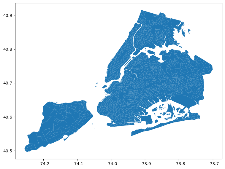
Now with the nyc object ready to go, here a few tasks for you to complete:

• Create a contiguity matrix using the queen criterion

• Let’s focus on Central Park. The corresponding polygon is ID 142. How many neighbors does it have?

• Try to reproduce the zoom plot in the previous section.

• Create a block spatial weights matrix where every tract is connected to other tracts in the same borough. For that, use the borocode column of the nyc table.

• Compare the number of neighbors by tract for the two weights matrices, which one has more? why?

Task II: Japanese cities

In this task, you will be generating spatial weights matrices based on distance. We will test your skills on this using a dataset of Japanese urban areas provided by OECD. Let’s get it ready for you to work on it directly.

If you are interested in the original methodology, you can check out in moreno2020metropolitan

The data is available over the web on this address but it is not accessible programmatically. For that reason, we have cached it on the data folder, and we can read it directly from there into a GeoDataFrame:

jp_cities = geopandas.read_file('../data/Japan.zip')
jp_cities.head()

	fuacode_si	fuaname	fuaname_en	class_code	iso3	name	geometry
0	JPN19	Kagoshima	Kagoshima	3.0	JPN	Japan	MULTIPOLYGON Z (((130.67888 31.62931 0.00000, ...
1	JPN20	Himeji	Himeji	3.0	JPN	Japan	MULTIPOLYGON Z (((134.51537 34.65958 0.00000, ...
2	JPN50	Hitachi	Hitachi	3.0	JPN	Japan	POLYGON Z ((140.58715 36.94447 0.00000, 140.61...
3	JPN08	Hiroshima	Hiroshima	3.0	JPN	Japan	MULTIPOLYGON Z (((132.29648 34.19932 0.00000, ...
4	JPN03	Toyota	Toyota	4.0	JPN	Japan	MULTIPOLYGON Z (((137.04096 34.73242 0.00000, ...

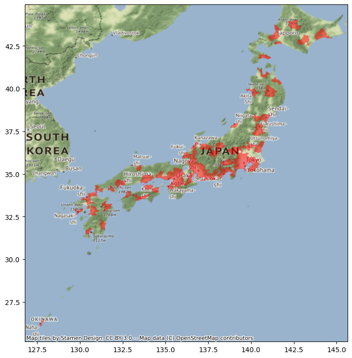
If we make a quick plot, we can see these are polygons covering the part of the Japanese geography that is considered urban by their analysis:

ax = jp_cities.plot(color="red", alpha=0.5, figsize=(9, 9))
contextily.add_basemap(ax, crs=jp_cities.crs)

For this example, we need two transformations: lon/lat coordinates to a geographical projection, and polygons to points. To calculate distances effectively, we need to ensure the coordinates of our geographic data are expressed in metres (or a similar measurement unit). The original dataset is expressed in lon/lat degrees:

jp_cities.crs

<Geographic 2D CRS: EPSG:4326>
Name: WGS 84
Axis Info [ellipsoidal]:
- Lat[north]: Geodetic latitude (degree)
- Lon[east]: Geodetic longitude (degree)
Area of Use:
- name: World.
- bounds: (-180.0, -90.0, 180.0, 90.0)
Datum: World Geodetic System 1984 ensemble
- Ellipsoid: WGS 84
- Prime Meridian: Greenwich

We can use the Japan Plane Rectangular CS XVII system (EPSG:2459), which is expressed in metres:

jp = jp_cities.to_crs(epsg=2459)

So the resulting table is in metres:

jp.crs

<Projected CRS: EPSG:2459>
Name: JGD2000 / Japan Plane Rectangular CS XVII
Axis Info [cartesian]:
- X[north]: Northing (metre)
- Y[east]: Easting (metre)
Area of Use:
- name: Japan - onshore Okinawa-ken east of 130°E.
- bounds: (131.12, 24.4, 131.38, 26.01)
Coordinate Operation:
- name: Japan Plane Rectangular CS zone XVII
- method: Transverse Mercator
Datum: Japanese Geodetic Datum 2000
- Ellipsoid: GRS 1980
- Prime Meridian: Greenwich

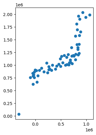
Now, distances are easier to calculate between points than between polygons. Hence, we will convert the urban areas into their centroids:

jp.geometry = jp.geometry.centroid

So the result is a seet of points expressed in metres:

jp.plot()

<Axes: >

With these at hand, tackle the following challenges:

• Generate a spatial weights matrix with five nearest neighbors

Tip

Remember the dataset is expressed in metres, not Kilometres!

• Generate a spatial weights matrix with a 100km distance band

• Compare the two in terms of average number of neighbors. What are the main differences you can spot? In which cases do you think one criterion would be preferable over the other?

Warning

The final task below is a bit more involved, so do not despair if you cannot get it to work completely!

Tip

Be careful with the projections you are using and make sure to plot every dataset in a figure in the same projection!

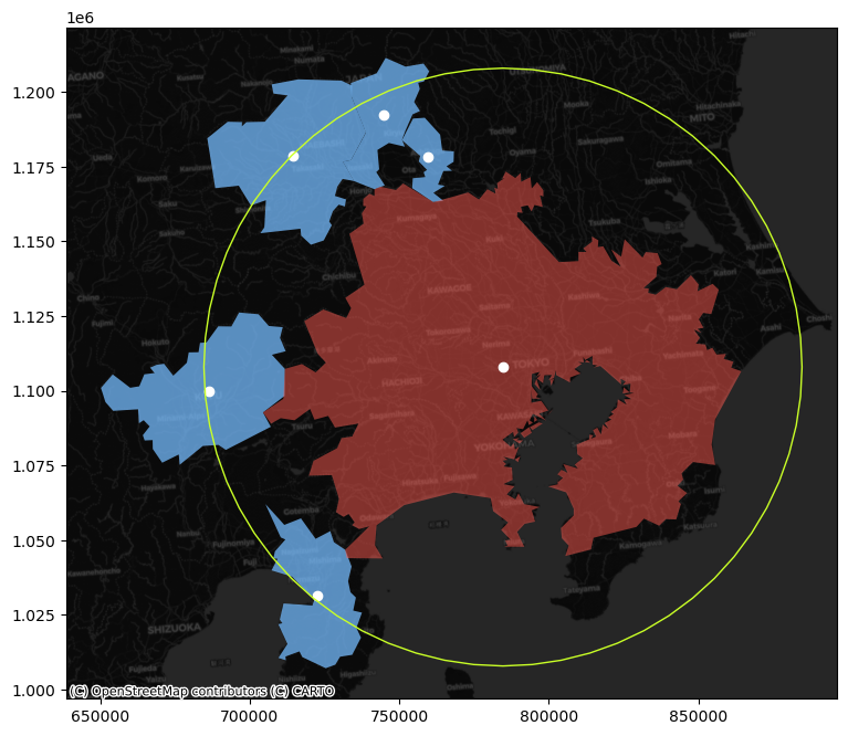
Focus on Tokyo (find the row in the table through a query search as we saw when considering Index-based queries) and the 100km spatial weights generated above. Try to create a figure similar to the one in the lecture. Here’s a recipe:

1. Generate a buffer of 100Km around the Tokyo centroid

2. Start the plot with the Tokyo urban area polygon (jp_cities) in one color (e.g. red)

3. Add its neighbors in, say blue

4. Add their centroids in a third different color

5. Layer on top the buffer, making sure only the edge is colored

6. [Optional] Add a basemap

If all goes well, your figure should look, more or less, like:

/opt/conda/lib/python3.10/site-packages/libpysal/weights/weights.py:172: UserWarning: The weights matrix is not fully connected: 
 There are 9 disconnected components.
 There are 4 islands with ids: 14, 17, 30, 54.
  warnings.warn(message)

Task III: Spatial Lag

Check out the notes on how to read the AHAH dataset on the DIY section of block D to refresh your mind before starting the task.

For this task, we will rely on the AHAH dataset. Create the spatial lag of the overall score, and generate a Moran plot. Can you tell any overall pattern? What do you think it means?