Supervised Learning
To do before…
Background
Here is a taster for supervised learning to make you want more, which we’ll do on the live session. To prepare for this part of the course (which includes the section below, as well as the one on inference and overfitting/CV), here are two tasks you will need to complete before the live session:
First, watch the following clip which sets up the scene for what will be to come
Second, read the following two articles, all mentioned in the clip:
Statistical Modeling: the Two Cultures ([B+01])
Machine Learning: An Applied Econometric Approach* ([MS17])
Regression trees
Most of this block relies on linear regression. Linear regression is one of the simplest but also most powerful supervised algorithms. Later in the section, we will contrast its use with another technique that has gained much popularity since its inception at the turn of the millenium: random forests. A detailed understanding of random forests goes beyond the scope of this course. However, its intuition will be useful and will be covered here.
To understand random forests, we first need to learn about regression trees:
A forest is no more than a collection of trees. A random forest thus will “grow” several trees, and then aggregate the predictions of each into a single, better prediction. This is what we call “bagging”:
Building on these two ideas, the notion of a “random” forest makes a bit more sense:
Action!
%matplotlib inline
from IPython.display import Image

import pandas
import numpy as np
Assuming you have the file downloaded on the path ../data/:
db = pandas.read_csv("../data/paris_abb.csv.zip")
If you’re online, you can do:
db = pandas.read_csv("https://github.com/darribas/data_science_studio/raw/master/content/data/paris_abb.csv.zip")
Linear Regression
The Econometrician way
import statsmodels.formula.api as sm
Raw price
f = "Price ~ bathrooms + bedrooms + room_type"
lm_raw = sm.ols(f, db)\
       .fit()
lm_raw
<statsmodels.regression.linear_model.RegressionResultsWrapper at 0x7f458e6d1cd0>
lm_raw.summary()
| Dep. Variable: | Price | R-squared: | 0.103 |
|---|---|---|---|
| Model: | OLS | Adj. R-squared: | 0.103 |
| Method: | Least Squares | F-statistic: | 1151. |
| Date: | Thu, 07 Jan 2021 | Prob (F-statistic): | 0.00 |
| Time: | 17:24:33 | Log-Likelihood: | -3.2312e+05 |
| No. Observations: | 50280 | AIC: | 6.462e+05 |
| Df Residuals: | 50274 | BIC: | 6.463e+05 |
| Df Model: | 5 | ||
| Covariance Type: | nonrobust |
| coef | std err | t | P>|t| | [0.025 | 0.975] | |
|---|---|---|---|---|---|---|
| Intercept | 69.3589 | 1.295 | 53.573 | 0.000 | 66.821 | 71.896 |
| room_type[T.Hotel room] | 148.7074 | 4.779 | 31.120 | 0.000 | 139.341 | 158.073 |
| room_type[T.Private room] | -51.5793 | 2.202 | -23.425 | 0.000 | -55.895 | -47.264 |
| room_type[T.Shared room] | -71.5010 | 8.692 | -8.226 | 0.000 | -88.537 | -54.465 |
| bathrooms | -2.4081 | 1.367 | -1.762 | 0.078 | -5.087 | 0.271 |
| bedrooms | 43.3410 | 0.939 | 46.174 | 0.000 | 41.501 | 45.181 |
| Omnibus: | 135133.909 | Durbin-Watson: | 1.923 |
|---|---|---|---|
| Prob(Omnibus): | 0.000 | Jarque-Bera (JB): | 6632879884.203 |
| Skew: | 32.680 | Prob(JB): | 0.00 |
| Kurtosis: | 1781.140 | Cond. No. | 27.2 |
Notes:
[1] Standard Errors assume that the covariance matrix of the errors is correctly specified.
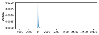
Now, \(Price\) is rather skewed:
db.Price.plot.kde(figsize=(6, 2));
We could take the log to try to obtain a better fit:
f = "np.log1p(Price) ~ bathrooms + bedrooms + room_type"
lm_log = sm.ols(f, db)\
       .fit()
lm_log
<statsmodels.regression.linear_model.RegressionResultsWrapper at 0x7f458e1484c0>
lm_log.rsquared
0.31515872008420753
lm_raw.rsquared
0.10269412705703151
That ☝️ is inference though. We’re here to “machine learn”!
# Get predictions
yp_raw = lm_raw.fittedvalues
yp_raw.head()
0     66.950833
1     66.950833
2    153.632865
3    110.291849
4    110.291849
dtype: float64
Or…
lm_raw.predict(db[["bathrooms",
                   "bedrooms",
                   "room_type"
                  ]])\
      .head()
0     66.950833
1     66.950833
2    153.632865
3    110.291849
4    110.291849
dtype: float64
The Machine Learner way
We need to:
Get the dummies ourselves first
room_type_ds = pandas.get_dummies(db["room_type"])
room_type_ds.head(2)
| Entire home/apt | Hotel room | Private room | Shared room | |
|---|---|---|---|---|
| 0 | 1 | 0 | 0 | 0 |
| 1 | 1 | 0 | 0 | 0 |
Prep
Xandy
X = pandas.concat([db[["bathrooms", "bedrooms"]],
                   room_type_ds.drop("Entire home/apt",
                                     axis=1)
                  ], axis=1
                 )
X.head()
| bathrooms | bedrooms | Hotel room | Private room | Shared room | |
|---|---|---|---|---|---|
| 0 | 1.0 | 0.0 | 0 | 0 | 0 |
| 1 | 1.0 | 0.0 | 0 | 0 | 0 |
| 2 | 1.0 | 2.0 | 0 | 0 | 0 |
| 3 | 1.0 | 1.0 | 0 | 0 | 0 |
| 4 | 1.0 | 1.0 | 0 | 0 | 0 |
Set up a model
from sklearn.linear_model import LinearRegression

regressor = LinearRegression()
Train the model (see the use of
fit)
regressor.fit(X, db["Price"])
LinearRegression()
And voila, we have our results!
pandas.Series(regressor.coef_,
              index=X.columns
             )
bathrooms        -2.408064
bedrooms         43.341016
Hotel room      148.707387
Private room    -51.579347
Shared room     -71.501010
dtype: float64
regressor.intercept_
69.35889717336228
lm_raw.params
Intercept                     69.358897
room_type[T.Hotel room]      148.707387
room_type[T.Private room]    -51.579347
room_type[T.Shared room]     -71.501010
bathrooms                     -2.408064
bedrooms                      43.341016
dtype: float64
Tree-based approaches: the Random Forest
from sklearn.ensemble import RandomForestRegressor
Very similar API (as throughout sklearn). Two parameters to set (see here for guidance):
rf_raw = RandomForestRegressor(n_estimators=100,
                               max_features=None
                              )

%time rf_raw.fit(X, db["Price"])
CPU times: user 750 ms, sys: 0 ns, total: 750 ms
Wall time: 749 ms
RandomForestRegressor(max_features=None)
To recover the predictions, we need to rely on predict:
rf_raw_lbls = rf_raw.predict(X)
rf_raw_lbls
array([ 71.98778067,  71.98778067, 140.74061093, ...,  93.62649936,
        71.98778067,  93.62649936])
For completeness, let’s quickly fit a Random Forest on the log of price:
rf_log = RandomForestRegressor(n_estimators=100,
                               max_features=None
                              )

%time rf_log.fit(X, np.log1p(db["Price"]))

rf_log_lbls = rf_log.predict(X)
CPU times: user 590 ms, sys: 0 ns, total: 590 ms
Wall time: 589 ms
EXERCISE
Train a random forest on the price using the number of beds and the property type instead
Before we move on, let’s record all the predictions in a single table for convenience:
res = pandas.DataFrame({"LM-Raw": lm_raw.fittedvalues,
                        "LM-Log": lm_log.fittedvalues,
                        "RF-Raw": rf_raw_lbls,
                        "RF-Log": rf_log_lbls,
                        "Truth": db["Price"]
                       })
res.head()
| LM-Raw | LM-Log | RF-Raw | RF-Log | Truth | |
|---|---|---|---|---|---|
| 0 | 66.950833 | 4.198030 | 71.987781 | 4.181397 | 60.0 |
| 1 | 66.950833 | 4.198030 | 71.987781 | 4.181397 | 115.0 |
| 2 | 153.632865 | 4.850742 | 140.740611 | 4.817468 | 119.0 |
| 3 | 110.291849 | 4.524386 | 93.626499 | 4.444683 | 130.0 |
| 4 | 110.291849 | 4.524386 | 93.626499 | 4.444683 | 75.0 |
And write it out to a file:
res.to_parquet("../data/lm_results.parquet")
An example with categorical outcomes
Let’s bring back the classification we did in the previous session:
k5_pca = pandas.read_parquet("../data/k5_pca.parquet")\
               .reindex(db.index)
k5_pca.head()
| k5_pca | |
|---|---|
| 0 | 2 |
| 1 | 1 |
| 2 | 0 |
| 3 | 2 |
| 4 | 2 |
Now we might conceive cases where we want to build a model to predict these classes based on some house characteristics. To illustrate it, let’s consider the same variables as above. In this case, however, we want a classifier rather than a regressor, as the response is categorical.
from sklearn.ensemble import RandomForestClassifier
But the training is very similar:
%%time

classifier = RandomForestClassifier(n_estimators=100,
                                    max_features="sqrt"
                                   )
classifier.fit(X, k5_pca["k5_pca"])

pred_lbls = pandas.Series(classifier.predict(X),
                          index=k5_pca.index
                         )
CPU times: user 1.23 s, sys: 0 ns, total: 1.23 s
Wall time: 1.23 s
class_res = pandas.DataFrame({"Truth": k5_pca["k5_pca"],
                              "Predicted": pred_lbls
                             }
                            ).apply(pandas.Categorical)
class_res.describe()
| Truth | Predicted | |
|---|---|---|
| count | 50280 | 50280 |
| unique | 5 | 5 |
| top | 2 | 2 |
| freq | 22773 | 49801 |