Inference
%matplotlib inline
from IPython.display import Image

import pandas
import numpy as np
import seaborn as sns
import matplotlib.pyplot as plt
import statsmodels.formula.api as sm
from sklearn.preprocessing import scale
from sklearn import metrics
Assuming you have the file downloaded on the path ../data/:
db = pandas.read_csv("../data/paris_abb.csv.zip")
If you’re online, you can do:
db = pandas.read_csv("https://github.com/darribas/data_science_studio/raw/master/content/data/paris_abb.csv.zip")
db['l_price'] = np.log1p(db['Price'])
db.info()
<class 'pandas.core.frame.DataFrame'>
RangeIndex: 50280 entries, 0 to 50279
Data columns (total 11 columns):
 #   Column                  Non-Null Count  Dtype
---  ------                  --------------  -----
 0   id                      50280 non-null  int64
 1   neighbourhood_cleansed  50280 non-null  object
 2   property_type           50280 non-null  object
 3   room_type               50280 non-null  object
 4   accommodates            50280 non-null  int64
 5   bathrooms               50280 non-null  float64
 6   bedrooms                50280 non-null  float64
 7   beds                    50280 non-null  float64
 8   bed_type                50280 non-null  object
 9   Price                   50280 non-null  float64
 10  l_price                 50280 non-null  float64
dtypes: float64(5), int64(2), object(4)
memory usage: 4.2+ MB
Baseline model
\(X\):
Bathrooms
Bedrooms
Beds
Room type
m1 = sm.ols('l_price ~ bedrooms + bathrooms + beds', db).fit()
m1.summary()
| Dep. Variable: | l_price | R-squared: | 0.245 |
|---|---|---|---|
| Model: | OLS | Adj. R-squared: | 0.245 |
| Method: | Least Squares | F-statistic: | 5433. |
| Date: | Thu, 07 Jan 2021 | Prob (F-statistic): | 0.00 |
| Time: | 17:25:24 | Log-Likelihood: | -38592. |
| No. Observations: | 50280 | AIC: | 7.719e+04 |
| Df Residuals: | 50276 | BIC: | 7.723e+04 |
| Df Model: | 3 | ||
| Covariance Type: | nonrobust |
| coef | std err | t | P>|t| | [0.025 | 0.975] | |
|---|---|---|---|---|---|---|
| Intercept | 4.1806 | 0.005 | 852.126 | 0.000 | 4.171 | 4.190 |
| bedrooms | 0.2253 | 0.004 | 57.760 | 0.000 | 0.218 | 0.233 |
| bathrooms | -0.1544 | 0.005 | -32.373 | 0.000 | -0.164 | -0.145 |
| beds | 0.1398 | 0.003 | 50.554 | 0.000 | 0.134 | 0.145 |
| Omnibus: | 11384.882 | Durbin-Watson: | 1.846 |
|---|---|---|---|
| Prob(Omnibus): | 0.000 | Jarque-Bera (JB): | 585415.122 |
| Skew: | -0.096 | Prob(JB): | 0.00 |
| Kurtosis: | 19.715 | Cond. No. | 7.94 |
Notes:
[1] Standard Errors assume that the covariance matrix of the errors is correctly specified.
To note:
Decent \(R^2\) (although that’s not holy truth)
Every variable significant and related as expected
Interpret coefficients
cols = ['bedrooms', 'bathrooms', 'beds']
scX = pandas.DataFrame(scale(db[cols]),
                       index=db.index,
                       columns=cols)
scX.describe()
| bedrooms | bathrooms | beds | |
|---|---|---|---|
| count | 5.028000e+04 | 5.028000e+04 | 5.028000e+04 |
| mean | 1.748138e-14 | 1.621070e-15 | -5.895298e-15 |
| std | 1.000010e+00 | 1.000010e+00 | 1.000010e+00 |
| min | -1.076738e+00 | -1.625116e+00 | -1.429042e+00 |
| 25% | -7.772733e-02 | -1.702805e-01 | -5.706025e-01 |
| 50% | -7.772733e-02 | -1.702805e-01 | -5.706025e-01 |
| 75% | -7.772733e-02 | -1.702805e-01 | 2.878366e-01 |
| max | 4.887380e+01 | 7.111664e+01 | 4.149292e+01 |
m2 = sm.ols('l_price ~ bedrooms + bathrooms + beds',
            data=scX.join(db['l_price']))\
       .fit()
m2.summary()
| Dep. Variable: | l_price | R-squared: | 0.245 |
|---|---|---|---|
| Model: | OLS | Adj. R-squared: | 0.245 |
| Method: | Least Squares | F-statistic: | 5433. |
| Date: | Thu, 07 Jan 2021 | Prob (F-statistic): | 0.00 |
| Time: | 17:25:24 | Log-Likelihood: | -38592. |
| No. Observations: | 50280 | AIC: | 7.719e+04 |
| Df Residuals: | 50276 | BIC: | 7.723e+04 |
| Df Model: | 3 | ||
| Covariance Type: | nonrobust |
| coef | std err | t | P>|t| | [0.025 | 0.975] | |
|---|---|---|---|---|---|---|
| Intercept | 4.4837 | 0.002 | 1928.462 | 0.000 | 4.479 | 4.488 |
| bedrooms | 0.2255 | 0.004 | 57.760 | 0.000 | 0.218 | 0.233 |
| bathrooms | -0.1061 | 0.003 | -32.373 | 0.000 | -0.113 | -0.100 |
| beds | 0.1628 | 0.003 | 50.554 | 0.000 | 0.156 | 0.169 |
| Omnibus: | 11384.882 | Durbin-Watson: | 1.846 |
|---|---|---|---|
| Prob(Omnibus): | 0.000 | Jarque-Bera (JB): | 585415.122 |
| Skew: | -0.096 | Prob(JB): | 0.00 |
| Kurtosis: | 19.715 | Cond. No. | 3.11 |
Notes:
[1] Standard Errors assume that the covariance matrix of the errors is correctly specified.
Let’s bring both sets of results together:
pandas.DataFrame({"Baseline": m1.params,
                  "X Std.": m2.params
                 })
| Baseline | X Std. | |
|---|---|---|
| Intercept | 4.180599 | 4.483657 |
| bedrooms | 0.225325 | 0.225548 |
| bathrooms | -0.154385 | -0.106119 |
| beds | 0.139759 | 0.162806 |
To note:
How does interpretation of the coefficients change?
Meaning of intecept when \(X\) is demeanded
Units in which \(\beta\) are interpreted
Predictive checking
Is the model picking up the overall “shape of data”?
Important to know how much we should trust our inferences
Crucial if we want to use the model to predict!
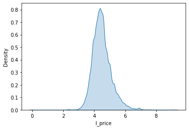
sns.kdeplot(db['l_price'], shade=True)
<AxesSubplot:xlabel='l_price', ylabel='Density'>
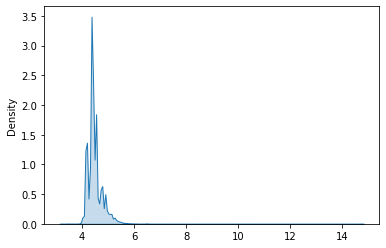
sns.kdeplot(m1.fittedvalues, shade=True)
<AxesSubplot:ylabel='Density'>
f, ax = plt.subplots(1, figsize=(9, 6))
sns.kdeplot(db['l_price'], shade=True, ax=ax, label='$y$')
sns.kdeplot(m1.fittedvalues, shade=True, ax=ax, label='$\hat{y}$')
plt.show()
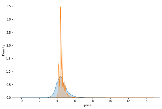
To note:
Not a terrible start
How could we improve it?
m3 = sm.ols('l_price ~ bedrooms + bathrooms + beds + room_type', db).fit()
m3.summary()
| Dep. Variable: | l_price | R-squared: | 0.340 |
|---|---|---|---|
| Model: | OLS | Adj. R-squared: | 0.340 |
| Method: | Least Squares | F-statistic: | 4314. |
| Date: | Thu, 07 Jan 2021 | Prob (F-statistic): | 0.00 |
| Time: | 17:25:25 | Log-Likelihood: | -35210. |
| No. Observations: | 50280 | AIC: | 7.043e+04 |
| Df Residuals: | 50273 | BIC: | 7.050e+04 |
| Df Model: | 6 | ||
| Covariance Type: | nonrobust |
| coef | std err | t | P>|t| | [0.025 | 0.975] | |
|---|---|---|---|---|---|---|
| Intercept | 4.2417 | 0.005 | 899.941 | 0.000 | 4.232 | 4.251 |
| room_type[T.Hotel room] | 0.5548 | 0.016 | 35.619 | 0.000 | 0.524 | 0.585 |
| room_type[T.Private room] | -0.4862 | 0.007 | -66.604 | 0.000 | -0.501 | -0.472 |
| room_type[T.Shared room] | -1.0320 | 0.028 | -36.320 | 0.000 | -1.088 | -0.976 |
| bedrooms | 0.2388 | 0.004 | 65.134 | 0.000 | 0.232 | 0.246 |
| bathrooms | -0.1440 | 0.004 | -32.285 | 0.000 | -0.153 | -0.135 |
| beds | 0.1144 | 0.003 | 43.386 | 0.000 | 0.109 | 0.120 |
| Omnibus: | 11695.728 | Durbin-Watson: | 1.878 |
|---|---|---|---|
| Prob(Omnibus): | 0.000 | Jarque-Bera (JB): | 680804.847 |
| Skew: | -0.027 | Prob(JB): | 0.00 |
| Kurtosis: | 21.027 | Cond. No. | 37.2 |
Notes:
[1] Standard Errors assume that the covariance matrix of the errors is correctly specified.
f, ax = plt.subplots(1, figsize=(9, 6))
sns.kdeplot(db['l_price'], shade=True, ax=ax, label='$y$')
sns.kdeplot(m1.fittedvalues, shade=True, ax=ax, label='$\hat{y}_1$')
sns.kdeplot(m3.fittedvalues, shade=True, ax=ax, label='$\hat{y}_2$')
plt.show()
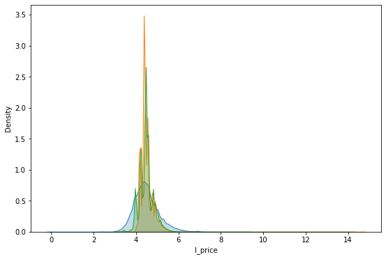
To note:
This is better!
But these are only point predictions. Sometimes that’s good enough.
Usually however, we want a model to capture the underlying process instead of the particular realisation observed (ie. dataset).
Then we need to think about the uncertainty embedded in the model we are estimating
Inferential Vs Predictive uncertainty
[See more in Chapter 7.2 of Gelman & Hill 2006 👌💯]
Two types of uncertainty in our model
Predictive (\(\epsilon\))
Inferential (\(\beta\))
Both affect the final predictions we make
Image("../figs/abb_room.png", retina=True)
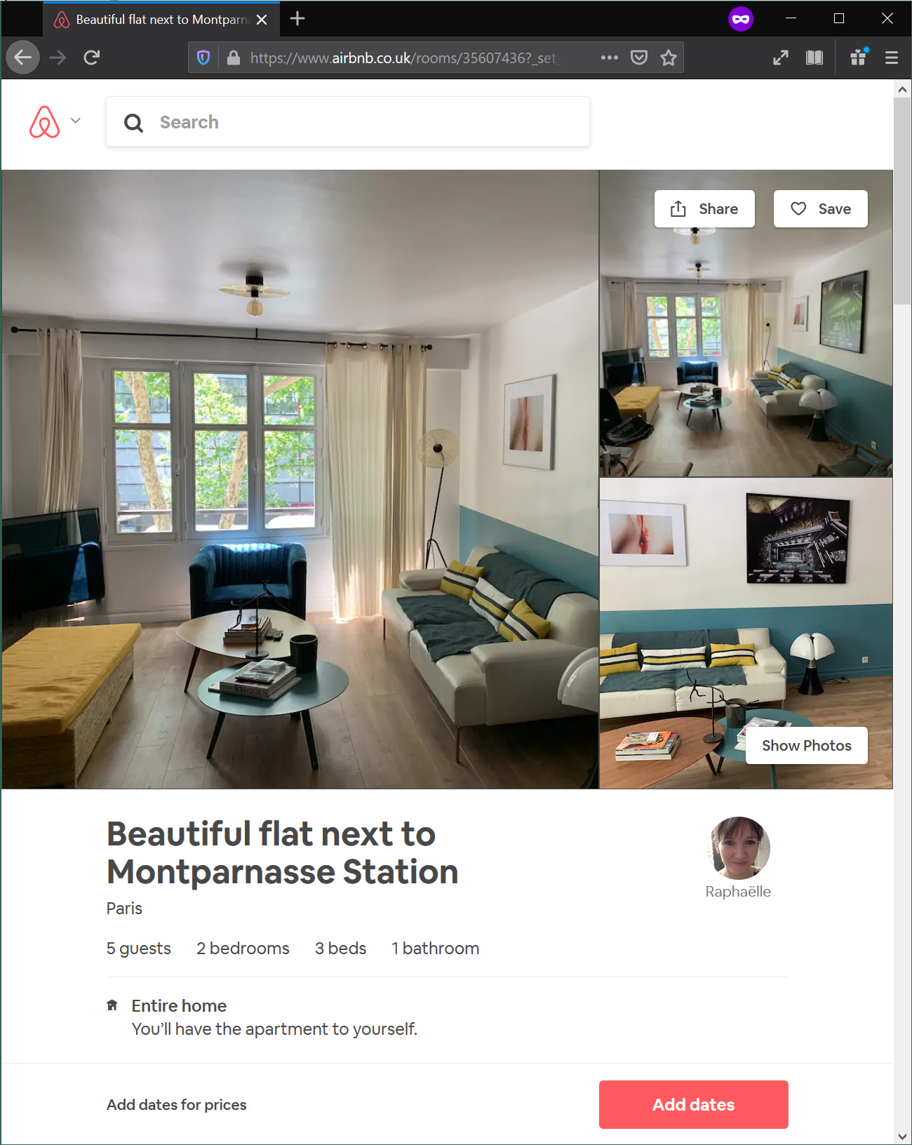
room = db.loc[db['id']==35607436, :]
room.T
| 45979 | |
|---|---|
| id | 35607436 |
| neighbourhood_cleansed | Luxembourg |
| property_type | Apartment |
| room_type | Entire home/apt |
| accommodates | 5 |
| bathrooms | 1 |
| bedrooms | 2 |
| beds | 3 |
| bed_type | Real Bed |
| Price | 90 |
| l_price | 4.51086 |
rid = room.index[0]
db.loc[rid, :]
id                               35607436
neighbourhood_cleansed         Luxembourg
property_type                   Apartment
room_type                 Entire home/apt
accommodates                            5
bathrooms                               1
bedrooms                                2
beds                                    3
bed_type                         Real Bed
Price                                  90
l_price                           4.51086
Name: 45979, dtype: object
m1.params['Intercept'] + db.loc[rid, cols].dot(m1.params[cols])
4.896141184855212
To note:
What does
dotdo?
m1.fittedvalues[rid]
4.896141184855212
Point predictive simulation
%%time
# Parameters
## Number of simulations
r = 2000
# Pull out characteristics for house of interest
x_i = db.loc[rid, cols]
# Specify model engine
model = m1

# Place-holder
sims = np.zeros(r)
# Loop over number of replications
for i in range(r):
    # Get a random draw of betas
    rbs = np.random.normal(model.params, model.bse)
    # Get a random draw of epsilon
    re = np.random.normal(0, model.scale)
    # Obtain point estimate
    y_hr = rbs[0] + np.dot(x_i, rbs[1:]) + re
    # Store estimate
    sims[i] = y_hr
CPU times: user 637 ms, sys: 35.1 ms, total: 672 ms
Wall time: 632 ms
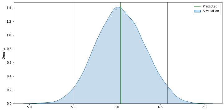
f, ax = plt.subplots(1, figsize=(12, 6))

sns.kdeplot(sims, shade=True, ax=ax, label='Simulation')
ax.axvline(db.loc[rid, 'l_price'], c='orange', label='Observed')
ax.axvline(model.fittedvalues[rid], c='green', label='Predicted')

lo, up = pandas.Series(sims)\
               .sort_values()\
               .iloc[[int(np.round(0.025 * r)), int(np.round(0.975 * r))]]
ax.axvline(lo, c='grey', linewidth=1)
ax.axvline(up, c='grey', linewidth=1)

plt.legend()
plt.show()
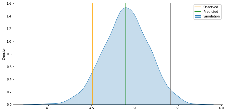
To note:
Intuition of the simulation
The
forloop, deconstructedThe graph, bit by bit
If we did this for every observation, we’d expect 95% to be within the 95% bands
Exercise
Explore with the code above and try to generate similar plots for:
Different houses across locations and characteristics
Different model
Exercise+
Recreate the analysis above for observation 5389821. What happens? Why?
Now, we could do this for all the observations and get a sense of the overall distribution to be expected
%%time
# Parameters
## Number of observations & simulations
n = db.shape[0]
r = 200
# Specify model engine
model = m1

# Place-holder (N, r)
sims = np.zeros((n, r))
# Loop over number of replications
for i in range(r):
    # Get a random draw of betas
    rbs = np.random.normal(model.params, model.bse)
    # Get a random draw of epsilon
    re = np.random.normal([0]*n, model.scale)
    # Obtain point estimate
    y_hr = rbs[0] + np.dot(db[cols], rbs[1:]) + re
    # Store estimate
    sims[:, i] = y_hr
CPU times: user 5.61 s, sys: 27.3 s, total: 32.9 s
Wall time: 2.08 s
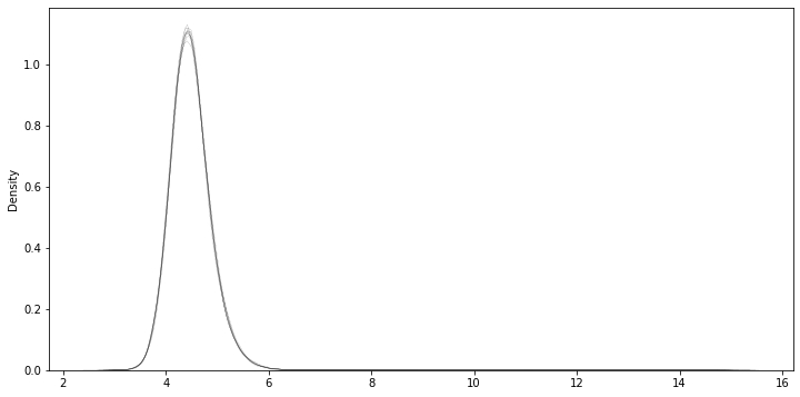
f, ax = plt.subplots(1, figsize=(12, 6))

for i in range(10):
    sns.kdeplot(sims[:, i], ax=ax, linewidth=0.1, alpha=0.1, color='k')

plt.show()
f, ax = plt.subplots(1, figsize=(12, 6))

sns.kdeplot(db['l_price'], shade=True, ax=ax, label='$y$')
sns.kdeplot(m1.fittedvalues, shade=True, ax=ax, label='$\hat{y}$')

for i in range(r):
    sns.kdeplot(sims[:, i], ax=ax, linewidth=0.1, alpha=0.1, color='k')

plt.show()
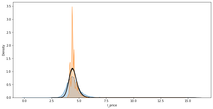
To note:
Black line contains
rthin lines that collectively capture the uncertainty behind the model
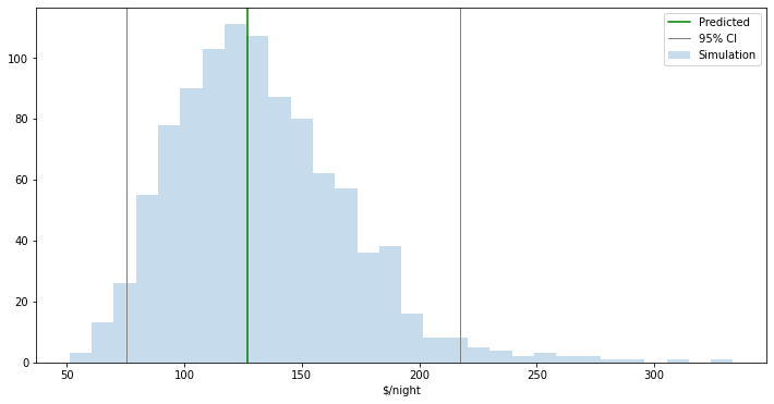
New data
Imagine we are trying to figure out how much should we charge for a property we want to put on AirBnb.
For example, let’s assume our property is:
new = pandas.Series({'bedrooms': 4,
                     'bathrooms': 1,
                     'beds': 8})
%%time
# Parameters
## Number of simulations
r = 2000
# Pull out characteristics for house of interest
x_i = new
# Specify model engine
model = m1

# Place-holder
sims = np.zeros(r)
# Loop over number of replications
for i in range(r):
    # Get a random draw of betas
    rbs = np.random.normal(model.params, model.bse)
    # Get a random draw of epsilon
    re = np.random.normal(0, model.scale)
    # Obtain point estimate
    y_hr = rbs[0] + np.dot(x_i, rbs[1:]) + re
    # Store estimate
    sims[i] = y_hr
CPU times: user 640 ms, sys: 4.53 ms, total: 644 ms
Wall time: 643 ms
f, ax = plt.subplots(1, figsize=(12, 6))

sns.kdeplot(sims, shade=True, ax=ax, label='Simulation')
ax.axvline(model.params.iloc[0] + np.dot(new, model.params.iloc[1:]), \
           c='green', label='Predicted')

lo, up = pandas.Series(sims)\
               .sort_values()\
               .iloc[[int(np.round(0.025 * r)), int(np.round(0.975 * r))]]
ax.axvline(lo, c='grey', linewidth=1)
ax.axvline(up, c='grey', linewidth=1)

plt.legend()
plt.show()
[Pro]
def predictor(bedrooms, bathrooms, beds):
    new = pandas.Series({'bedrooms': bedrooms,
                         'bathrooms': bathrooms,
                         'beds': beds
                        })
    r = 1000
    x_i = new
    model = m1
    y_hat = model.params.iloc[0] + np.dot(new, model.params.iloc[1:])
    # Simulation
    sims = np.zeros(r)
    for i in range(r):
        rbs = np.random.normal(model.params, model.bse)
        re = np.random.normal(0, model.scale)
        y_hr = rbs[0] + np.dot(x_i, rbs[1:]) + re
        sims[i] = y_hr
    sims = np.exp(sims)
    y_hat = np.exp(y_hat)
    # Bands
    lo, up = pandas.Series(sims)\
                   .sort_values()\
                   .iloc[[int(np.round(0.025 * r)), int(np.round(0.975 * r))]]
    # Setup'n'draw figure
    f, ax = plt.subplots(1, figsize=(12, 6))
    ax.hist(sims, label='Simulation', alpha=0.25, bins=30)
    ax.axvline(y_hat, c='green', label='Predicted')
    ax.axvline(lo, c='grey', linewidth=1, label='95% CI')
    ax.axvline(up, c='grey', linewidth=1)
    #ax.set_xlim((0, 10))
    # Dress up
    ax.set_xlabel("$/night")
    plt.legend()
    return plt.show()

predictor(3, 1, 1)
# You might have to run this to make interactives work
# jupyter labextension install @jupyter-widgets/jupyterlab-manager
# From https://ipywidgets.readthedocs.io/en/latest/user_install.html#installing-the-jupyterlab-extension
# Then restart Jupyter Lab
from ipywidgets import interact, IntSlider

interact(predictor,
         bedrooms=IntSlider(min=1, max=10), \
         bathrooms=IntSlider(min=0, max=10), \
         beds=IntSlider(min=1, max=20)
        );
Model performance
To note:
Switch from inference to prediction
Overall idea of summarising model performance
\(R^2\)
Error-based measures
# R^2
r2 = pandas.Series({'Baseline': metrics.r2_score(db['l_price'],
                                                 m1.fittedvalues),
                    'Augmented': metrics.r2_score(db['l_price'],
                                                  m3.fittedvalues)})
r2
Baseline     0.244826
Augmented    0.339876
dtype: float64
# MSE
mse = pandas.Series({'Baseline': metrics.mean_squared_error(db['l_price'],
                                                            m1.fittedvalues),
                     'Augmented': metrics.mean_squared_error(db['l_price'],
                                                             m3.fittedvalues)})
mse
Baseline     0.271771
Augmented    0.237565
dtype: float64
# MAE
mae = pandas.Series({'Baseline': metrics.mean_absolute_error(db['l_price'],
                                                             m1.fittedvalues),
                     'Augmented': metrics.mean_absolute_error(db['l_price'],
                                                              m3.fittedvalues)})
mae
Baseline     0.379119
Augmented    0.357287
dtype: float64
# All
perf = pandas.DataFrame({'MAE': mae,
                         'MSE': mse,
                         'R^2': r2})
perf
| MAE | MSE | R^2 | |
|---|---|---|---|
| Baseline | 0.379119 | 0.271771 | 0.244826 |
| Augmented | 0.357287 | 0.237565 | 0.339876 |