Do-It-Yourself#
import geopandas
import contextily
Task I: NYC Geodemographics#
We are going to try to get at the (geographic) essence of New York City. For that, we will rely on the same set up Census tracts for New York City we used a few blocks ago. Once you have the nyc object loaded, create a geodemographic classification using the following variables:
european: Total Population Whiteasian: Total Population Asian Americanamerican: Total Population American Indianafrican: Total Population African Americanhispanic: Total Population Hispanicmixed: Total Population Mixed racepacific: Total Population Pacific Islander
For this, make sure you standardise the table by the size of each tract. That is, compute a column with the total population as the sum of all the ethnic groups and divide each of them by that column. This way, the values will range between 0 (no population of a given ethnic group) and 1 (all the population in the tract is of that group).
Once this is ready, get to work with the following tasks:
Pick a number of clusters (e.g. 10)
Run K-Means for that number of clusters
Plot the different clusters on a map
Analyse the results:
What do you find?
What are the main characteristics of each cluster?
How are clusters distributed geographically?
Can you identify some groups concentrated on particular areas (e.g. China Town, Little Italy)?
Task II: Regionalisation of Dar Es Salaam#
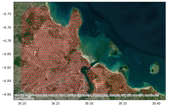
For this task we will travel to Tanzania’s Dar Es Salaam. We are using a dataset assembled to describe the built environment of the city centre. Let’s load up the dataset before anything:
# Read the file in
db = geopandas.read_file(
    "http://darribas.org/gds_course/content/data/dar_es_salaam.geojson"
)
Alternative
Instead of reading the file directly off the web, it is possible to download it manually, store it on your computer, and read it locally. To do that, you can follow these steps:
Download the file by right-clicking on this link and saving the file
Place the file on the same folder as the notebook where you intend to read it
Replace the code in the cell above by:
br = geopandas.read_file("dar_es_salaam.geojson")
Geographically, this is what we are looking at:
Show code cell source
ax = db.plot(
    facecolor="none",
    edgecolor="red",
    linewidth=0.5,
    figsize=(9, 9)
)
contextily.add_basemap(
    ax,
    crs=db.crs,
    source=contextily.providers.Esri.WorldImagery
);
We can inspect the table:
db.info()
<class 'geopandas.geodataframe.GeoDataFrame'>
RangeIndex: 1291 entries, 0 to 1290
Data columns (total 7 columns):
 #   Column             Non-Null Count  Dtype
---  ------             --------------  -----
 0   index              1291 non-null   object
 1   id                 1291 non-null   object
 2   street_length      1291 non-null   float64
 3   street_linearity   1291 non-null   float64
 4   building_density   1291 non-null   float64
 5   building_coverage  1291 non-null   float64
 6   geometry           1291 non-null   geometry
dtypes: float64(4), geometry(1), object(2)
memory usage: 70.7+ KB
Two main aspects of the built environment are considered: the street network and buildings. To capture those, the following variables are calculated at for the H3 hexagonal grid system, zoom level 8:
Building density: number of buildings per hexagon
Building coverage: proportion of the hexagon covered by buildings
Street length: total length of streets within the hexagon
Street linearity: a measure of how regular the street network is
With these at hand, your task is the following:
Develop a regionalisation that partitions Dar Es Salaam based on its built environment
For that, you can follow these suggestions:
Create a spatial weights matrix to capture spatial relationships between hexagons
Set up a regionalisation algorithm with a given number of clusters (e.g. seven)
Generate a geography that contains only the boundaries of each region and visualise it (ideally with a satellite image as basemap for context)
Rinse and repeat with several combinations of variables and number of clusters
Pick your best. Why have you selected it? What does it show? What are the main groups of areas based on the built environment?