Spatial Data
Contents
Spatial Data
📖 Ahead of time…
This block is all about understanding spatial data, both conceptually and practically. Before your fingers get on the keyboard, the following readings will help you get going and familiar with core ideas:
Chapter 1 of the GDS Book [RABWng], which provides a conceptual overview of representing Geography in data
Chapter 3 of the GDS Book [RABWng], a sister chapter with a more applied perspective on how concepts are implemented in computer data structures
Additionally, parts of this block are based and source from Block C in the GDS Course [AB19].
💻 Hands-on coding
(Geographic) tables
import pandas
import geopandas
import xarray, rioxarray
import contextily
import matplotlib.pyplot as plt
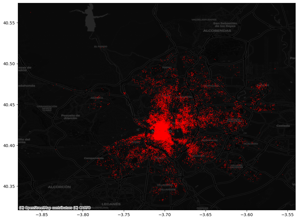
Points
Assuming you have the file locally on the path ../data/:
pts = geopandas.read_file("../data/madrid_abb.gpkg")
If you’re online, you can do:
pts = geopandas.read_file(
    "https://github.com/GDSL-UL/san/raw/v0.1.0/data/assignment_1_madrid/madrid_abb.gpkg"
)
Point geometries from columns
Sometimes, points are provided as separate columns in an otherwise non-spatial table. For example imagine we have an object cols which looks like:
cols.head()
          X         Y
0  0.259602  0.854351
1  0.661662  0.782427
2  0.932211  0.319130
3  0.395249  0.469885
4  0.303446  0.008525
In this case, we can convert those into proper geometries by:
pts = geopandas.GeoSeries(
    geopandas.points_from_xy(cols["X"], cols["Y"])
)
pts.info()
<class 'geopandas.geodataframe.GeoDataFrame'>
RangeIndex: 18399 entries, 0 to 18398
Data columns (total 16 columns):
 #   Column           Non-Null Count  Dtype
---  ------           --------------  -----
 0   price            18399 non-null  object
 1   price_usd        18399 non-null  float64
 2   log1p_price_usd  18399 non-null  float64
 3   accommodates     18399 non-null  int64
 4   bathrooms        18399 non-null  object
 5   bedrooms         18399 non-null  float64
 6   beds             18399 non-null  float64
 7   neighbourhood    18399 non-null  object
 8   room_type        18399 non-null  object
 9   property_type    18399 non-null  object
 10  WiFi             18399 non-null  object
 11  Coffee           18399 non-null  object
 12  Gym              18399 non-null  object
 13  Parking          18399 non-null  object
 14  km_to_retiro     18399 non-null  float64
 15  geometry         18399 non-null  geometry
dtypes: float64(5), geometry(1), int64(1), object(9)
memory usage: 2.2+ MB
pts.head()
| price | price_usd | log1p_price_usd | accommodates | bathrooms | bedrooms | beds | neighbourhood | room_type | property_type | WiFi | Coffee | Gym | Parking | km_to_retiro | geometry | |
|---|---|---|---|---|---|---|---|---|---|---|---|---|---|---|---|---|
| 0 | $60.00 | 60.0 | 4.110874 | 2 | 1 shared bath | 1.0 | 1.0 | Hispanoamérica | Private room | Private room in apartment | 1 | 0 | 0 | 0 | 5.116664 | POINT (-3.67688 40.45724) |
| 1 | $31.00 | 31.0 | 3.465736 | 1 | 1 bath | 1.0 | 1.0 | Cármenes | Private room | Private room in apartment | 1 | 1 | 0 | 1 | 5.563869 | POINT (-3.74084 40.40341) |
| 2 | $60.00 | 60.0 | 4.110874 | 6 | 2 baths | 3.0 | 5.0 | Legazpi | Entire home/apt | Entire apartment | 1 | 1 | 0 | 1 | 3.048442 | POINT (-3.69304 40.38695) |
| 3 | $115.00 | 115.0 | 4.753590 | 4 | 1.5 baths | 2.0 | 3.0 | Justicia | Entire home/apt | Entire apartment | 1 | 1 | 0 | 1 | 2.075484 | POINT (-3.69764 40.41995) |
| 4 | $26.00 | 26.0 | 3.295837 | 1 | 1 private bath | 1.0 | 1.0 | Legazpi | Private room | Private room in house | 1 | 0 | 0 | 0 | 2.648058 | POINT (-3.69011 40.38985) |
Challenge
Show the top ten values of of price and neighbourhood
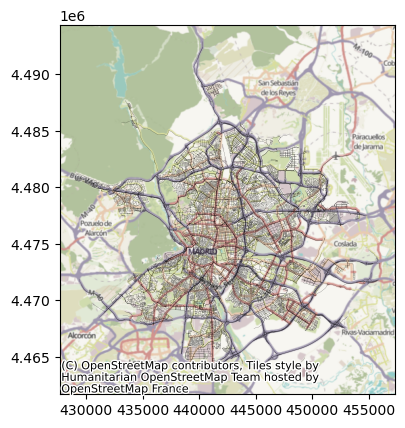
Lines
Assuming you have the file locally on the path ../data/:
pts = geopandas.read_file("../data/arturo_streets.gpkg")
If you’re online, you can do:
pts = geopandas.read_file(
    "https://darribas.org/gds4ae/_downloads/67d5480f98453027d59bf49606a7ad92/arturo_streets.gpkg"
)
lines.info()
<class 'geopandas.geodataframe.GeoDataFrame'>
RangeIndex: 66499 entries, 0 to 66498
Data columns (total 9 columns):
 #   Column              Non-Null Count  Dtype
---  ------              --------------  -----
 0   OGC_FID             66499 non-null  object
 1   dm_id               66499 non-null  object
 2   dist_barri          66483 non-null  object
 3   average_quality     66499 non-null  float64
 4   population_density  66499 non-null  float64
 5   X                   66499 non-null  float64
 6   Y                   66499 non-null  float64
 7   value               5465 non-null   float64
 8   geometry            66499 non-null  geometry
dtypes: float64(5), geometry(1), object(3)
memory usage: 4.6+ MB
lines.loc[0, "geometry"]

Challenge
Print descriptive statistics for population_density and average_quality
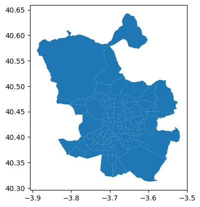
Polygons
Assuming you have the file locally on the path ../data/:
polys = geopandas.read_file("../data/neighbourhoods.geojson")
If you’re online, you can do:
polys = geopandas.read_file(
    "https://darribas.org/gds4ae/_downloads/44b4bc22c042386c2c0f8dc6685ef17c/neighbourhoods.geojson"
)
polys.head()
| neighbourhood | neighbourhood_group | geometry | |
|---|---|---|---|
| 0 | Palacio | Centro | MULTIPOLYGON (((-3.70584 40.42030, -3.70625 40... |
| 1 | Embajadores | Centro | MULTIPOLYGON (((-3.70384 40.41432, -3.70277 40... |
| 2 | Cortes | Centro | MULTIPOLYGON (((-3.69796 40.41929, -3.69645 40... |
| 3 | Justicia | Centro | MULTIPOLYGON (((-3.69546 40.41898, -3.69645 40... |
| 4 | Universidad | Centro | MULTIPOLYGON (((-3.70107 40.42134, -3.70155 40... |
polys.query("neighbourhood_group == 'Retiro'")
| neighbourhood | neighbourhood_group | geometry | |
|---|---|---|---|
| 13 | Pacífico | Retiro | MULTIPOLYGON (((-3.67015 40.40654, -3.67017 40... |
| 14 | Adelfas | Retiro | MULTIPOLYGON (((-3.67283 40.39468, -3.67343 40... |
| 15 | Estrella | Retiro | MULTIPOLYGON (((-3.66506 40.40647, -3.66512 40... |
| 16 | Ibiza | Retiro | MULTIPOLYGON (((-3.66916 40.41796, -3.66927 40... |
| 17 | Jerónimos | Retiro | MULTIPOLYGON (((-3.67874 40.40751, -3.67992 40... |
| 18 | Niño Jesús | Retiro | MULTIPOLYGON (((-3.66994 40.40850, -3.67012 40... |
polys.neighbourhood_group.unique()
array(['Centro', 'Arganzuela', 'Retiro', 'Salamanca', 'Chamartín',
       'Moratalaz', 'Tetuán', 'Chamberí', 'Fuencarral - El Pardo',
       'Moncloa - Aravaca', 'Puente de Vallecas', 'Latina', 'Carabanchel',
       'Usera', 'Ciudad Lineal', 'Hortaleza', 'Villaverde',
       'Villa de Vallecas', 'Vicálvaro', 'San Blas - Canillejas',
       'Barajas'], dtype=object)
Challenge
Print the neighborhoods within the “Latina” group
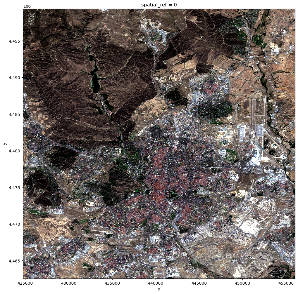
Surfaces
Assuming you have the file locally on the path ../data/:
sat = xarray.open_rasterio("../data/madrid_scene_s2_10_tc.tif")
If you’re online, you can do:
sat = xarray.open_rasterio(
    "https://darribas.org/gds4ae/_downloads/cafed4de0cfde63e6d2ffcb92264b431/madrid_scene_s2_10_tc.tif"
)
sat
<xarray.DataArray (band: 3, y: 3681, x: 3129)>
[34553547 values with dtype=uint8]
Coordinates:
  * band         (band) int64 1 2 3
  * x            (x) float64 4.248e+05 4.248e+05 4.248e+05 ... 4.56e+05 4.56e+05
  * y            (y) float64 4.499e+06 4.499e+06 ... 4.463e+06 4.463e+06
    spatial_ref  int64 0
Attributes:
    AREA_OR_POINT:  Area
    scale_factor:   1.0
add_offset: 0.0sat.sel(band=1)
<xarray.DataArray (y: 3681, x: 3129)>
[11517849 values with dtype=uint8]
Coordinates:
    band         int64 1
  * x            (x) float64 4.248e+05 4.248e+05 4.248e+05 ... 4.56e+05 4.56e+05
  * y            (y) float64 4.499e+06 4.499e+06 ... 4.463e+06 4.463e+06
    spatial_ref  int64 0
Attributes:
    AREA_OR_POINT:  Area
    scale_factor:   1.0
add_offset: 0.0sat.sel(
x=slice(430000, 440000), # x is ascending
y=slice(4480000, 4470000) # y is descending
)
<xarray.DataArray (band: 3, y: 1000, x: 1000)>
[3000000 values with dtype=uint8]
Coordinates:
  * band         (band) int64 1 2 3
  * x            (x) float64 4.3e+05 4.3e+05 4.3e+05 ... 4.4e+05 4.4e+05 4.4e+05
  * y            (y) float64 4.48e+06 4.48e+06 4.48e+06 ... 4.47e+06 4.47e+06
    spatial_ref  int64 0
Attributes:
    AREA_OR_POINT:  Area
    scale_factor:   1.0
add_offset: 0.0Challenge
Subset sat to band 2 and the section within [444444, 455555] of Easting and [4470000, 4480000] of Northing.
How many pixels does it contain?
What if you used bands 1 and 3 instead?
Visualisation
polys.explore()
polys.plot()
<Axes: >
ax = lines.plot(linewidth=0.1, color="black")
contextily.add_basemap(ax, crs=lines.crs)
ax = pts.plot(color="red", figsize=(12, 12), markersize=0.1)
contextily.add_basemap(
    ax,
    crs = pts.crs,
    source = contextily.providers.CartoDB.DarkMatter
);
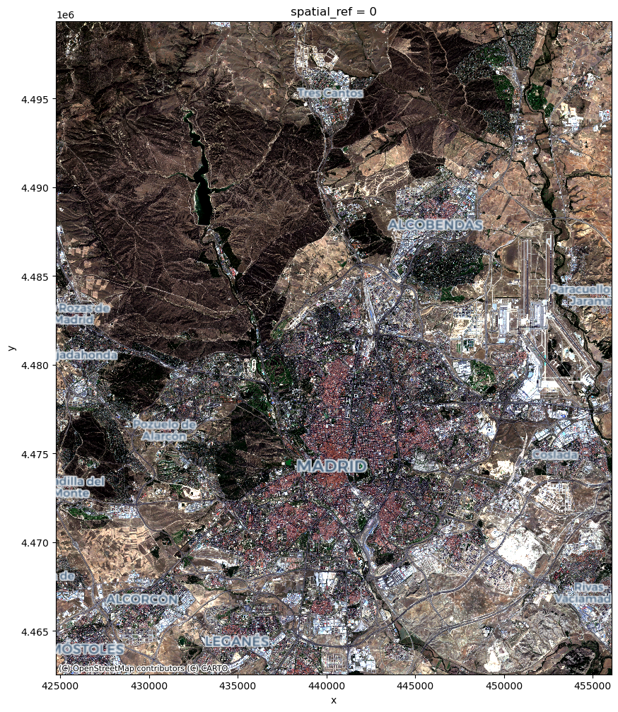
sat.plot.imshow(figsize=(12, 12))
<matplotlib.image.AxesImage at 0x7f7803bc36d0>
f, ax = plt.subplots(1, figsize=(12, 12))
sat.plot.imshow(ax=ax)
contextily.add_basemap(
    ax,
    crs=sat.rio.crs,
    source=contextily.providers.CartoDB.VoyagerOnlyLabels,
    zoom=11,
);
Challenge
Make three plots of sat, plotting one single band in each
Spatial operations
(Re-)Projections
pts.crs
<Geographic 2D CRS: EPSG:4326>
Name: WGS 84
Axis Info [ellipsoidal]:
- Lat[north]: Geodetic latitude (degree)
- Lon[east]: Geodetic longitude (degree)
Area of Use:
- name: World.
- bounds: (-180.0, -90.0, 180.0, 90.0)
Datum: World Geodetic System 1984 ensemble
- Ellipsoid: WGS 84
- Prime Meridian: Greenwich
sat.rio.crs
CRS.from_epsg(32630)
pts.to_crs(sat.rio.crs).crs
<Projected CRS: EPSG:32630>
Name: WGS 84 / UTM zone 30N
Axis Info [cartesian]:
- [east]: Easting (metre)
- [north]: Northing (metre)
Area of Use:
- undefined
Coordinate Operation:
- name: UTM zone 30N
- method: Transverse Mercator
Datum: World Geodetic System 1984
- Ellipsoid: WGS 84
- Prime Meridian: Greenwich
sat.rio.reproject(pts.crs).rio.crs
CRS.from_epsg(4326)
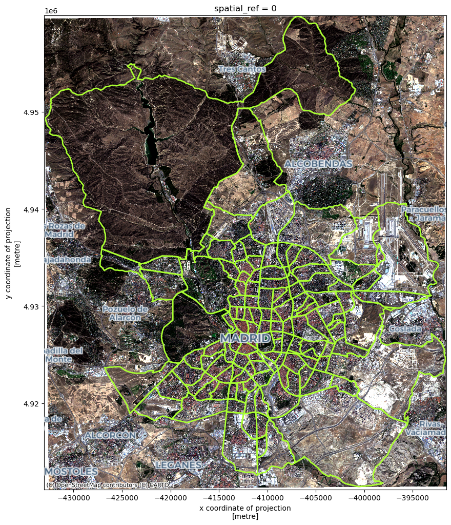
# All into Web Mercator (EPSG:3857)
f, ax = plt.subplots(1, figsize=(12, 12))
## Satellite image
sat.rio.reproject(
    "EPSG:3857"
).plot.imshow(
    ax=ax
)
## Neighbourhoods
polys.to_crs(epsg=3857).plot(
    linewidth=2,
    edgecolor="xkcd:lime",
    facecolor="none",
    ax=ax
)
## Labels
contextily.add_basemap( # No need to reproject
    ax,
    source=contextily.providers.CartoDB.VoyagerOnlyLabels,
);
Centroids
polys.centroid
/tmp/ipykernel_2058/2101097851.py:1: UserWarning: Geometry is in a geographic CRS. Results from 'centroid' are likely incorrect. Use 'GeoSeries.to_crs()' to re-project geometries to a projected CRS before this operation.

  polys.centroid
0      POINT (-3.71398 40.41543)
1      POINT (-3.70237 40.40925)
2      POINT (-3.69674 40.41485)
3      POINT (-3.69657 40.42367)
4      POINT (-3.70698 40.42568)
                 ...
123    POINT (-3.59135 40.45656)
124    POINT (-3.59723 40.48441)
125    POINT (-3.55847 40.47613)
126    POINT (-3.57889 40.47471)
127    POINT (-3.60718 40.46415)
Length: 128, dtype: geometry
lines.centroid
0        POINT (444133.737 4482808.936)
1        POINT (444192.064 4482878.034)
2        POINT (444134.563 4482885.414)
3        POINT (445612.661 4479335.686)
4        POINT (445606.311 4479354.437)
                      ...
66494    POINT (451980.378 4478407.920)
66495    POINT (436975.438 4473143.749)
66496    POINT (442218.600 4478415.561)
66497    POINT (442213.869 4478346.700)
66498    POINT (442233.760 4478278.748)
Length: 66499, dtype: geometry
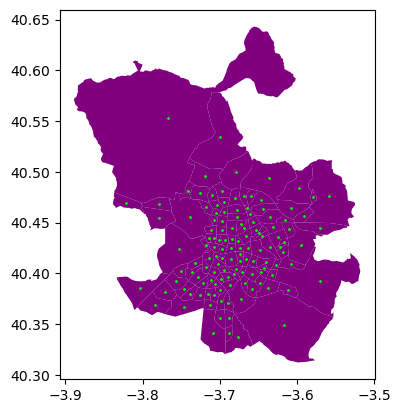
ax = polys.plot(color="purple")
polys.centroid.plot(
    ax=ax, color="lime", markersize=1
)
/tmp/ipykernel_2058/1054587808.py:2: UserWarning: Geometry is in a geographic CRS. Results from 'centroid' are likely incorrect. Use 'GeoSeries.to_crs()' to re-project geometries to a projected CRS before this operation.

  polys.centroid.plot(
<Axes: >
Spatial joins
sj = geopandas.sjoin(
    lines,
    polys.to_crs(lines.crs)
)
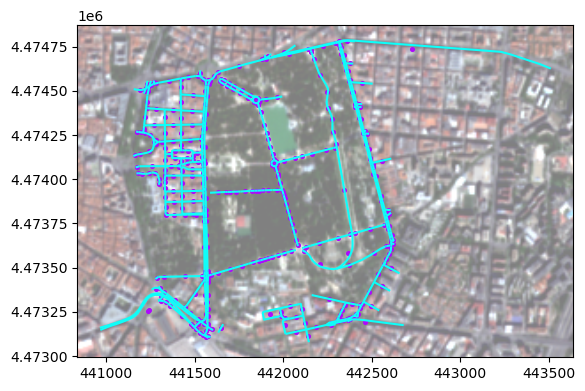
# Subset of lines
ax = sj.query(
    "neighbourhood == 'Jerónimos'"
).plot(color="xkcd:bright turquoise")

# Subset of line centroids
ax = sj.query(
    "neighbourhood == 'Jerónimos'"
).centroid.plot(
    color="xkcd:bright violet", markersize=7, ax=ax
)

# Local basemap
contextily.add_basemap(
    ax,
    crs=sj.crs,
    source="../data/madrid_scene_s2_10_tc.tif",
    alpha=0.5
)
sj.info()
<class 'geopandas.geodataframe.GeoDataFrame'>
Index: 69420 entries, 0 to 66438
Data columns (total 12 columns):
 #   Column               Non-Null Count  Dtype
---  ------               --------------  -----
 0   OGC_FID              69420 non-null  object
 1   dm_id                69420 non-null  object
 2   dist_barri           69414 non-null  object
 3   average_quality      69420 non-null  float64
 4   population_density   69420 non-null  float64
 5   X                    69420 non-null  float64
 6   Y                    69420 non-null  float64
 7   value                5769 non-null   float64
 8   geometry             69420 non-null  geometry
 9   index_right          69420 non-null  int64
 10  neighbourhood        69420 non-null  object
 11  neighbourhood_group  69420 non-null  object
dtypes: float64(5), geometry(1), int64(1), object(5)
memory usage: 6.9+ MB
Areas
areas = polys.to_crs(
    epsg=25830
).area * 1e-6 # Km2
areas.head()
0    1.471037
1    1.033253
2    0.592049
3    0.742031
4    0.947616
dtype: float64
Distances
cemfi = geopandas.tools.geocode(
    "Calle Casado del Alisal, 5, Madrid"
).to_crs(epsg=25830)
cemfi
| geometry | address | |
|---|---|---|
| 0 | POINT (441477.245 4473939.537) | 5, Calle Casado del Alisal, 28014, Calle Casad... |
polys.to_crs(
    cemfi.crs
).distance(
    cemfi.geometry
)
/tmp/ipykernel_2058/176561454.py:1: UserWarning: The indices of the two GeoSeries are different.
  polys.to_crs(
0      1491.338749
1              NaN
2              NaN
3              NaN
4              NaN
          ...
123            NaN
124            NaN
125            NaN
126            NaN
127            NaN
Length: 128, dtype: float64
d2cemfi = polys.to_crs(
    cemfi.crs
).distance(
    cemfi.geometry[0] # NO index
)
d2cemfi.head()
0    1491.338749
1     565.418135
2     278.121017
3     650.926572
4    1196.771601
dtype: float64
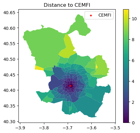
ax = polys.assign(
    dist=d2cemfi/1000
).plot("dist", legend=True)

cemfi.to_crs(
    polys.crs
).plot(
    marker="*",
    markersize=15,
    color="r",
    label="CEMFI",
    ax=ax
)

ax.legend()
ax.set_title(
    "Distance to CEMFI"
);
Challenge
Give Task III in this block of the GDS course a go
🐾 Next steps
If you are interested in following up on some of the topics explored in this block, the following pointers might be useful:
Although we have seen here
geopandasonly, all non-geographic operations on geo-tables are really thanks topandas, the workhorse for tabular data in Python. Their official documentation is an excellent first stop. If you prefer a book, McKinney (2012) [McK12] is a great one.For more detail on geographic operations on geo-tables, the Geopandas official documentation is a great place to continue the journey.
Surfaces, as covered here, are really an example of multi-dimensional labelled arrays. The library we use,
xarrayrepresents the cutting edge for working with these data structures in Python, and their documentation is a great place to wrap your head around how data of this type can be manipulated. For geographic extensions (CRS handling, reprojections, etc.), we have usedrioxarrayunder the hood, and its documentation is also well worth checking.