Where in the UK do neighbouring small areas look most unlike each other from space? This notebook measures dissimilarity between contiguous LSOAs (and their Scottish/NI equivalents) using the distance between their 2024 AlphaEarth satellite-embedding vectors, aggregated by Imago.
Setup
The libraries used throughout: geopandas for the polygons and embeddings, libpysal’s new Graph for contiguity, scikit-learn for cosine distances, and joblib to compute them in parallel. autoreload picks up edits to the shared gdsl30dmc_tools.py module without restarting the kernel.
code
%load_ext autoreload%autoreload 2import numpy as npimport pandas as pdimport geopandas as gpdimport matplotlib.pyplot as pltfrom joblib import Parallel, delayedfrom libpysal import graphfrom sklearn.metrics.pairwise import paired_cosine_distancesprint(gpd.__version__)
1.2.0
Reading data
Imago ships one GeoPackage per year, each holding small-area polygons (British National Grid, EPSG:27700) alongside the mean of each of the 64 embedding bands within the area. We start with 2024 and split the attributes into an embedding matrix for later distance calculations.
code
YEAR =2024lsoas = gpd.read_file(f"data/extracted-lsoa-geopackage_{YEAR}_output.gpkg")band_cols = [c for c in lsoas.columns if c.startswith("band")]lsoas = lsoas.set_index("data_zone_code")print(lsoas.crs, lsoas.shape)lsoas.index.str[0].value_counts().rename({"E": "England", "W": "Wales", "S": "Scotland", "N": "N. Ireland"})
ERROR 1: PROJ: proj_create_from_database: Open of /opt/conda/envs/gds/share/proj failed
EPSG:27700 (46844, 65)
data_zone_code
England       33755
Scotland       7392
N. Ireland     3780
Wales          1917
Name: count, dtype: int64
count    46844.000000
mean         0.910100
std          0.034245
min          0.747833
25%          0.885152
50%          0.911380
75%          0.937016
max          0.992520
dtype: float64
Building the contiguity graph
We connect areas that share at least one boundary point (queen contiguity) using the new libpysal.graph.Graph API, keeping all four nations. Since the polygons come from four national statistical agencies, we first try the standard builder and check how many links cross national borders, where boundaries may not line up.
Only one England–Scotland pair is linked, even though about two dozen pairs of areas meet along that border. The two nations’ polygons slightly overlap there (by up to ~70,000 m²), and contiguity only counts polygons that touch without overlapping. Fuzzy contiguity links any pair of geometries that intersect, which covers touching (queen) and overlapping polygons alike, so it fixes the border without adding spurious links elsewhere.
code
%%timeg = graph.Graph.build_fuzzy_contiguity(lsoas)edges =lambda g: set(g.adjacency[g.adjacency >0].index)print("Links only in queen:", len(edges(g_queen) - edges(g)), "| only in fuzzy:", len(edges(g) - edges(g_queen)))link_types(g)
Links only in queen: 0 | only in fuzzy: 42
CPU times: user 3.38 s, sys: 32.1 ms, total: 3.41 s
Wall time: 3.41 s
count    46844.000000
mean         5.816455
std          2.323981
min          0.000000
25%          4.000000
50%          6.000000
75%          7.000000
max         53.000000
Name: cardinalities, dtype: float64
Dropping areas with no neighbours
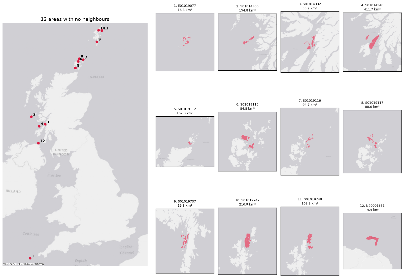
Note: the 12 areas with no neighbours (their own islands, with no link to any other area) are removed from both the graph and the embeddings table at this point, because a neighbour-dissimilarity score is undefined without neighbours. Island groups made up of several areas (e.g. in the Hebrides or Orkney) are kept, since their areas still neighbour each other. Everything below works on the trimmed g, lsoas and emb.
The figure below records which areas were dropped, before we remove them: all 12 are offshore islands (Scilly, the Inner Hebrides, Orkney, Shetland and Rathlin), not mainland areas the graph wrongly failed to link.
We measure how different each area is from each of its neighbours using cosine distance between their 2024 embedding vectors (1 − cosine similarity, from 0 for identical directions to 2 for opposite). Cosine ignores vector length, which in these area averages partly reflects how mixed the land cover is, and is the comparison AlphaEarth embeddings are designed for. Neighbours come from the fuzzy-contiguity graph g, i.e. queen contiguity plus the overlapping England–Scotland border pairs.
The 46,832 areas are split into 16 groups (one per core), and each group’s distances to all its neighbours are computed on a separate thread. NumPy releases Python’s global interpreter lock while it computes, so threads share the arrays without copying them. The results are reassembled into the order of g.adjacency and stored as the weights of a new graph, g_dist.
code
%%timeN_CHUNKS =16emb = np.ascontiguousarray(emb) # row-major, so gathering whole rows is fast (~4x here)adj = g.adjacencyi = lsoas.index.get_indexer(adj.index.get_level_values("focal")) # row of each focal area in embj = lsoas.index.get_indexer(adj.index.get_level_values("neighbor"))# Assign each area to one of N_CHUNKS groups, then find the links whose focal area is in each grouparea_chunk = np.repeat(np.arange(N_CHUNKS), [len(c) for c in np.array_split(np.arange(len(lsoas)), N_CHUNKS)])link_chunk = area_chunk[i]rows = [np.flatnonzero(link_chunk == k) for k inrange(N_CHUNKS)]parts = Parallel(n_jobs=N_CHUNKS, backend="threading")( delayed(paired_cosine_distances)(emb[i[r]], emb[j[r]]) for r in rows)dist = np.empty(len(adj))for r, d inzip(rows, parts): dist[r] = dg_dist = graph.Graph(pd.Series(dist, index=adj.index, name="weight"))
CPU times: user 1.12 s, sys: 271 ms, total: 1.39 s
Wall time: 865 ms
code
# Sanity checks: every link covered once, identical to the serial calculation, same structure as gassertsum(len(r) for r in rows) ==len(adj)assert np.allclose(dist, paired_cosine_distances(emb[i], emb[j]))assert g_dist.n_edges == g.n_edges and (g_dist.unique_ids == g.unique_ids).all()g_dist.adjacency.describe()
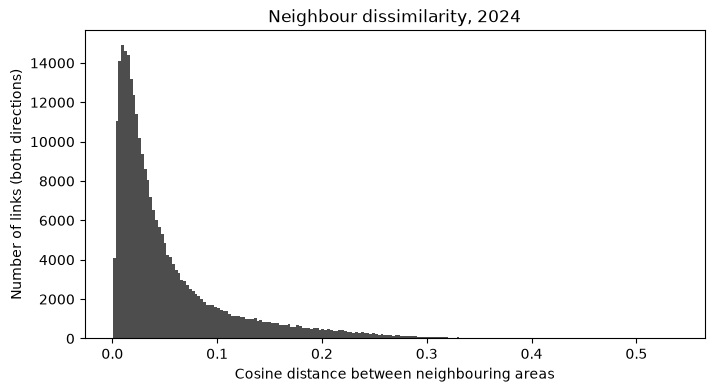
count    272466.000000
mean          0.053723
std           0.058251
min           0.000446
25%           0.015623
50%           0.032057
75%           0.068060
max           0.538219
Name: weight, dtype: float64
code
fig, ax = plt.subplots(figsize=(8, 4))ax.hist(g_dist.adjacency, bins=200, color="0.3")ax.set_xlabel("Cosine distance between neighbouring areas")ax.set_ylabel("Number of links (both directions)")ax.set_title(f"Neighbour dissimilarity, {YEAR}");
Most dissimilar neighbour
For each area we keep the single neighbour it differs from most, and the cosine distance to it. The result is a table with one row per area, indexed by area code, with two columns: neighbor (the most dissimilar neighbour’s code) and distance.
code
d = g_dist.adjacencymost_dissimilar = ( d.sort_values(ascending=False) .reset_index() .drop_duplicates("focal") # keeps each area's largest distance .set_index("focal") .reindex(lsoas.index) .rename(columns={"weight": "distance"}))most_dissimilar.index.name ="area"assert most_dissimilar.notna().all().all()most_dissimilar.sort_values("distance", ascending=False).head(10)
neighbor
distance
area
E01030710
E01030745
0.538219
E01030745
E01030710
0.538219
E01030744
E01030745
0.535450
E01030746
E01030745
0.533737
E01030711
E01030745
0.524066
E01031353
E01031359
0.513233
E01031359
E01031353
0.513233
E01034298
E01020936
0.502896
E01020936
E01034298
0.502896
E01030708
E01030745
0.502224
code
most_dissimilar["distance"].describe()
count    46832.000000
mean         0.116488
std          0.076095
min          0.001527
25%          0.056489
50%          0.099182
75%          0.162252
max          0.538219
Name: distance, dtype: float64
Dissimilarity from the whole neighbourhood
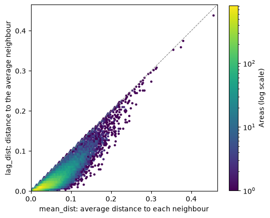
Two ways to score how different an area is from its neighbourhood as a whole, using equal weights for every neighbour:
mean_dist: the average of the cosine distances to each neighbour, i.e. how different the area is from its neighbours one by one. Taken from the weights of g_dist.
lag_dist: the cosine distance to the average neighbour, i.e. how different the area is from its surroundings taken together. The average neighbour is the spatial lag of the embeddings on the row-standardised graph.
Since averaging neighbours tends to cancel out their differences, lag_dist should be at most mean_dist for nearly every area. The gap between the two is roughly how much the neighbours differ among themselves.
code
emb_lag = g.transform("r").lag(emb) # row i = mean embedding of area i's neighboursneighbourhood = pd.DataFrame({"mean_dist": g_dist.aggregate("mean").reindex(lsoas.index),"lag_dist": paired_cosine_distances(emb, emb_lag),}, index=lsoas.index)assert neighbourhood.notna().all().all()print("Areas where lag_dist > mean_dist:", (neighbourhood.lag_dist > neighbourhood.mean_dist).sum())print("Spearman rank correlation:", round(neighbourhood.corr(method="spearman").iloc[0, 1], 3))neighbourhood.describe()
Areas where lag_dist > mean_dist: 0
Spearman rank correlation: 0.839
mean_dist
lag_dist
count
46832.000000
46832.000000
mean
0.053231
0.025731
std
0.033342
0.026431
min
0.001246
0.000389
25%
0.029067
0.009408
50%
0.046407
0.017330
75%
0.069374
0.032247
max
0.455714
0.438115
code
fig, ax = plt.subplots(figsize=(6, 6))hb = ax.hexbin(neighbourhood.mean_dist, neighbourhood.lag_dist, gridsize=120, bins="log", cmap="viridis", mincnt=1)lim = neighbourhood.max().max() *1.02ax.plot([0, lim], [0, lim], color="0.5", lw=0.8, ls="--")ax.set_xlim(0, lim); ax.set_ylim(0, lim); ax.set_aspect("equal")ax.set_xlabel("mean_dist: average distance to each neighbour")ax.set_ylabel("lag_dist: distance to the average neighbour")fig.colorbar(hb, ax=ax, shrink=0.8, label="Areas (log scale)");
Mapping the most dissimilar areas
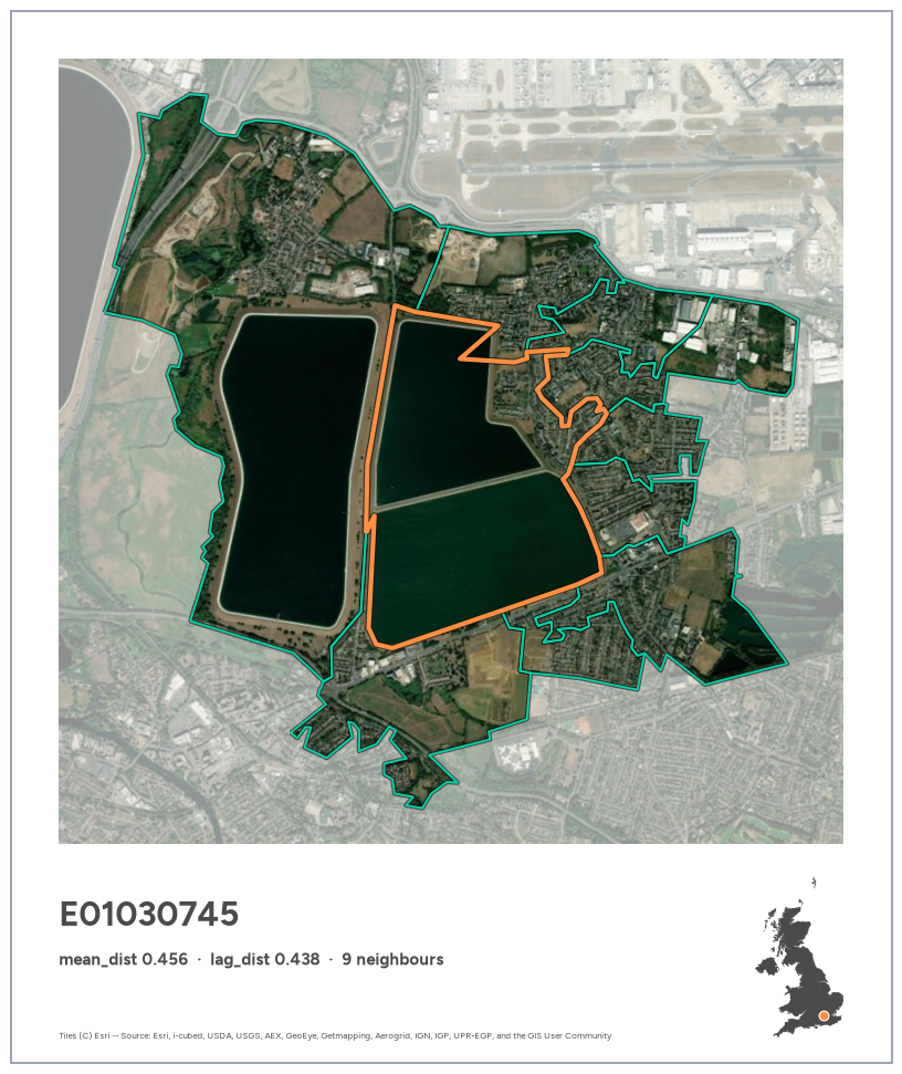
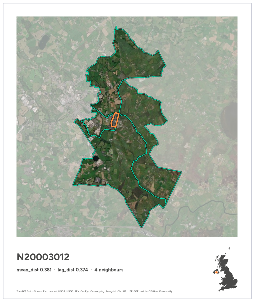
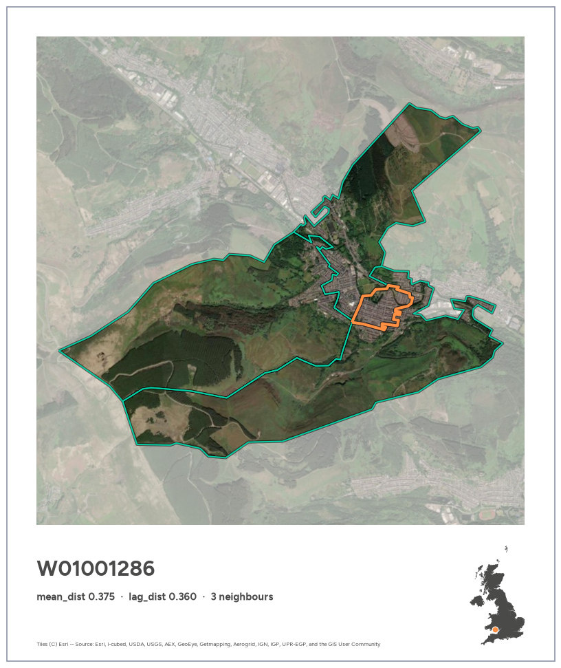
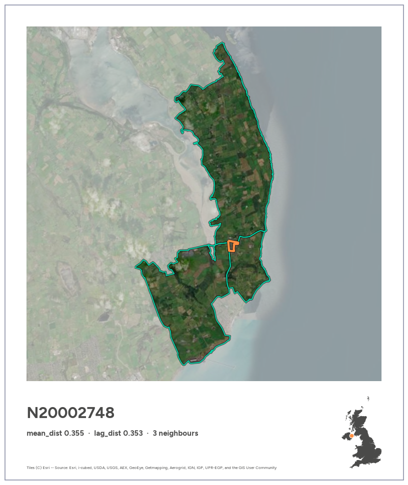
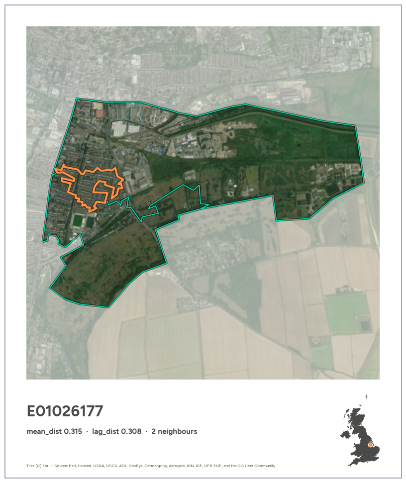
Each area becomes a Polaroid-style card. A square satellite photo (Esri imagery, no API key needed) shows the focal area outlined in orange and its neighbours in green, with everything outside them washed out towards white. Below it, a caption strip carries the area code and its scores in bold Figtree, Imago’s brand font, plus a UK silhouette locating the area. Colours follow Imago’s brand palette: Orange #FF8F42, Green #03CEA3, and Imago Grey #4A4A49 for the text and the UK silhouette.
The card template, the UK silhouette and the export helper live in gdsl30dmc_tools.py, shared with the other notebooks. The silhouette is built by merging each nation’s areas, using GEOS’s fast coverage_union where the polygons tile cleanly, then simplifying. It takes about 25 s and is cached to data/uk_outline.parquet, so it’s only built once.
code
%%timeimport gdsl30dmc_tools as toolsuk_outline = tools.uk_outline(lsoas)
CPU times: user 25.7 s, sys: 510 ms, total: 26.2 s
Wall time: 26.2 s
code
def plot_focal(code):"""Card for area `code` (orange) and its neighbours (green), captioned with its neighbourhood scores.""" s = neighbourhood.loc[code] subtitle =f"mean_dist {s.mean_dist:.3f} · lag_dist {s.lag_dist:.3f} · {g.cardinalities[code]} neighbours"return tools.area_card(lsoas, code, g.neighbors[code], subtitle, uk_outline)def plot_pair(a, b):"""Card for neighbouring areas `a` (orange) and `b` (green), captioned with their cosine distance.""" subtitle =f"cosine distance {g_dist.adjacency.loc[(a, b)]:.3f} · neighbouring areas"return tools.pair_card(lsoas, a, b, subtitle, uk_outline)
The most dissimilar area
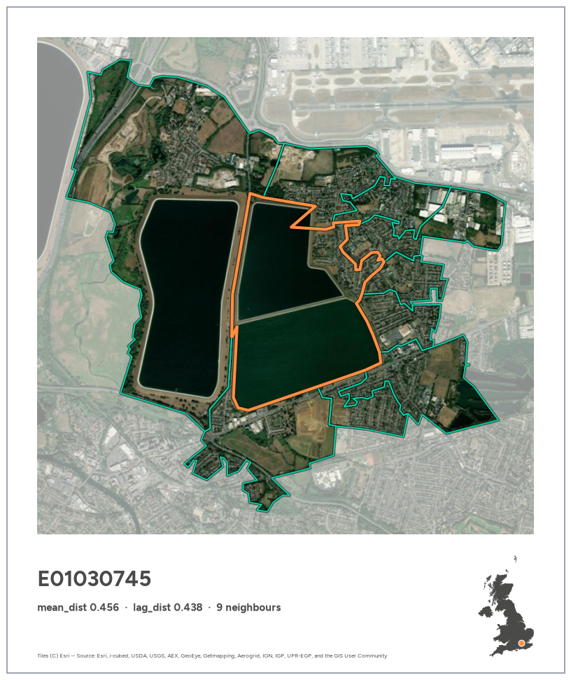
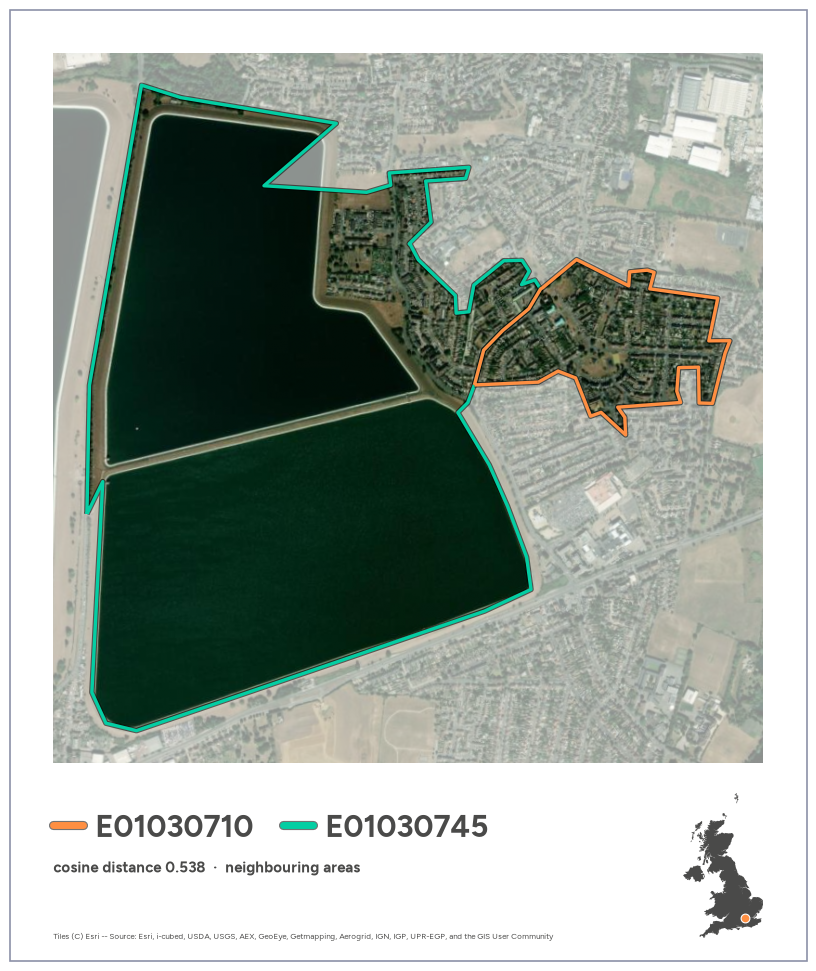
E01030745 ranks first on both mean_dist and lag_dist. It is almost entirely open water, a pair of reservoir basins just south of Heathrow, surrounded by housing, industry and airport land. Its only similar neighbour (cosine distance 0.16) is the large reservoir to the west.
code
top = neighbourhood["lag_dist"].idxmax()assert top == neighbourhood["mean_dist"].idxmax()fig = plot_focal(top)
Exporting the cards
Cards are saved to figures/ at 200 dpi with tools.export_card, keeping the full white border and caption strip. It doesn’t use bbox_inches="tight", which would trim the Polaroid margins.
We take the five highest-scoring areas on mean_dist and on lag_dist, combine them into one list without duplicates, and make and export a card for each. The table shows each area’s rank on both measures.
for code in cases: fig = plot_focal(code)print(export_card(fig, code)) plt.show()
/home/jovyan/work/figures/E01030745.png
/home/jovyan/work/figures/N20003012.png
/home/jovyan/work/figures/W01001286.png
/home/jovyan/work/figures/N20002748.png
/home/jovyan/work/figures/E01026177.png
Most dissimilar neighbouring pairs
Instead of scoring an area against its whole neighbourhood, we now look at individual pairs of neighbours: two areas that share a border and look most unlike each other from space. Each pair appears twice in g_dist (A→B and B→A, with the same distance), so we keep one row per pair and rank them by cosine distance.
count    136233.000000
mean          0.053723
std           0.058251
min           0.000446
25%           0.015623
50%           0.032057
75%           0.068060
max           0.538219
Name: distance, dtype: float64
code
top_pairs = pairs.head(20)print("Distinct areas among the top 20 pairs:", pd.unique(top_pairs[["area_a", "area_b"]].values.ravel()).size)print("Most frequent areas in the top 20:")print(pd.Series(top_pairs[["area_a", "area_b"]].values.ravel()).value_counts().head(5).to_string())top_pairs
Distinct areas among the top 20 pairs: 32
Most frequent areas in the top 20:
E01030745    7
E01034298    2
N20003012    2
E01030744    1
E01030711    1
area_a
area_b
distance
0
E01030710
E01030745
0.538219
1
E01030744
E01030745
0.535450
2
E01030745
E01030746
0.533737
3
E01030711
E01030745
0.524066
4
E01031353
E01031359
0.513233
5
E01020936
E01034298
0.502896
6
E01030708
E01030745
0.502224
7
E01020937
E01034298
0.501605
8
E01029178
E01035125
0.483857
9
W01001947
W01002024
0.480610
10
E01032000
E01032002
0.478253
11
E01003806
E01003807
0.473121
12
E01016234
E01016236
0.472666
13
E01028757
E01035757
0.464131
14
E01030734
E01030745
0.462928
15
S01018583
S01018595
0.461067
16
N20003012
N20003016
0.459638
17
S01019753
S01019761
0.458229
18
E01030743
E01030745
0.457491
19
N20002993
N20003012
0.454623
Top distinct pairs
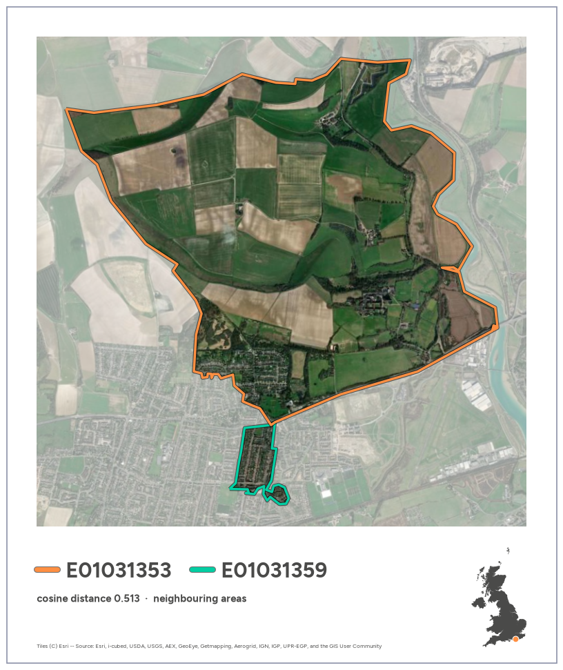
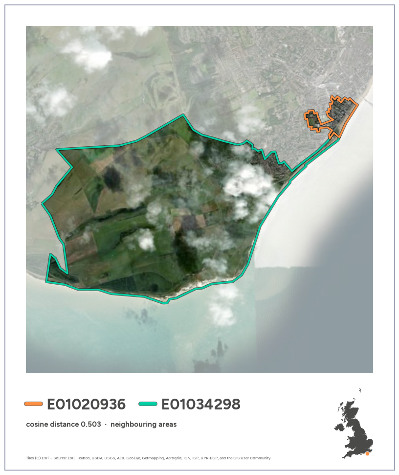
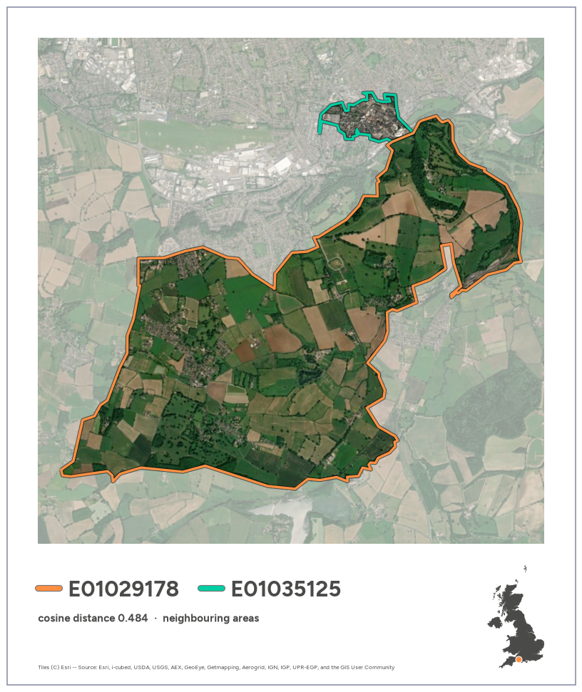
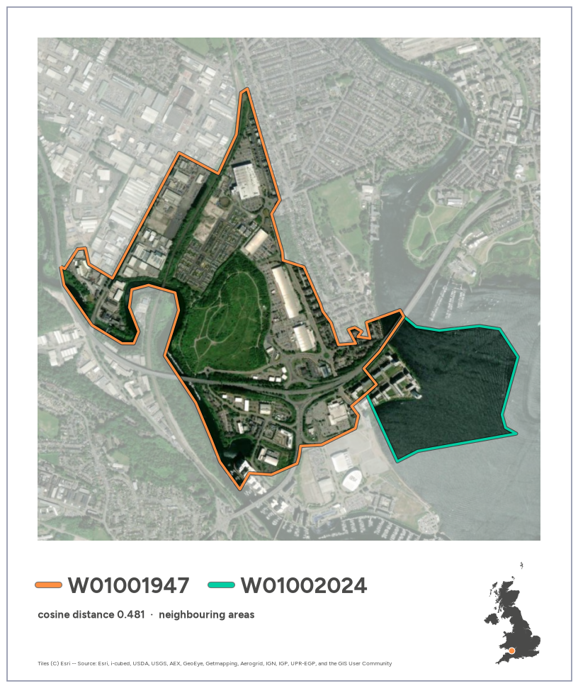
To avoid one area filling the list, we go down the ranking and skip any pair that shares an area with a pair already chosen. Each area then appears at most once. Each selected pair gets a Polaroid card from the same template as the area cards (polaroid(), via plot_pair): area A outlined in orange, area B in green, with a matching colour key next to each code in the caption.
code
N_PAIRS =5used, picks =set(), []for row in pairs.itertuples():if row.area_a in used or row.area_b in used:continue picks.append(row.Index) used |= {row.area_a, row.area_b}iflen(picks) == N_PAIRS:breaktop_distinct = pairs.loc[picks]top_distinct
area_a
area_b
distance
0
E01030710
E01030745
0.538219
4
E01031353
E01031359
0.513233
5
E01020936
E01034298
0.502896
8
E01029178
E01035125
0.483857
9
W01001947
W01002024
0.480610
code
for row in top_distinct.itertuples(): fig = plot_pair(row.area_a, row.area_b)print(export_card(fig, f"pair_{row.area_a}_{row.area_b}")) plt.show()