Get started with the GDS stack (Windows)
This document shows how you can get started with the tools used in the GDS'17 course. In particular, it walks you through each step of three of the most common tasks you will have to do in order to follow on each computer practical:
- Start the Jupyter Notebook
- Download notebook files with the practicals
- Download data files and access them within the notebook
We assume, you are either on a university computer that has all the required software installed (Install University Applications --> Scientific --> Geographic Data Science Stack 2017) or, if you are on a personal computer, you have installed all the software following the instructions (if not, go here).
Fire up the jupyter notebook
All of the course is based on the Jupyter notebook, a computational environment that provides an interface to the Python programming language by allowing to capture in a single document (an .ipynb file, or notebook from now on) Python code, its output, and additional text.
Follow these steps to start the notebook app:
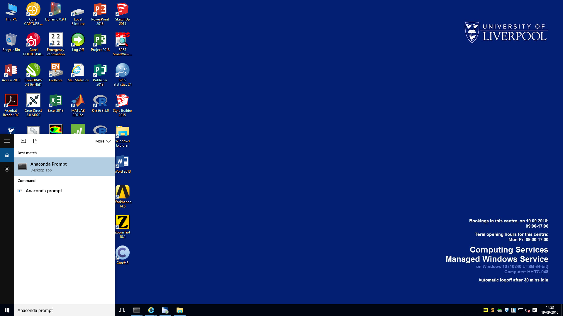
- Go to the
Search Windowsbox on the bottom-left corner of the screen and typeAnaconda Prompt(on Windows 7, this can be accessed through theStartmenu and "Search Programs and files"):
- Hit enter and that should open up a window that looks like this:
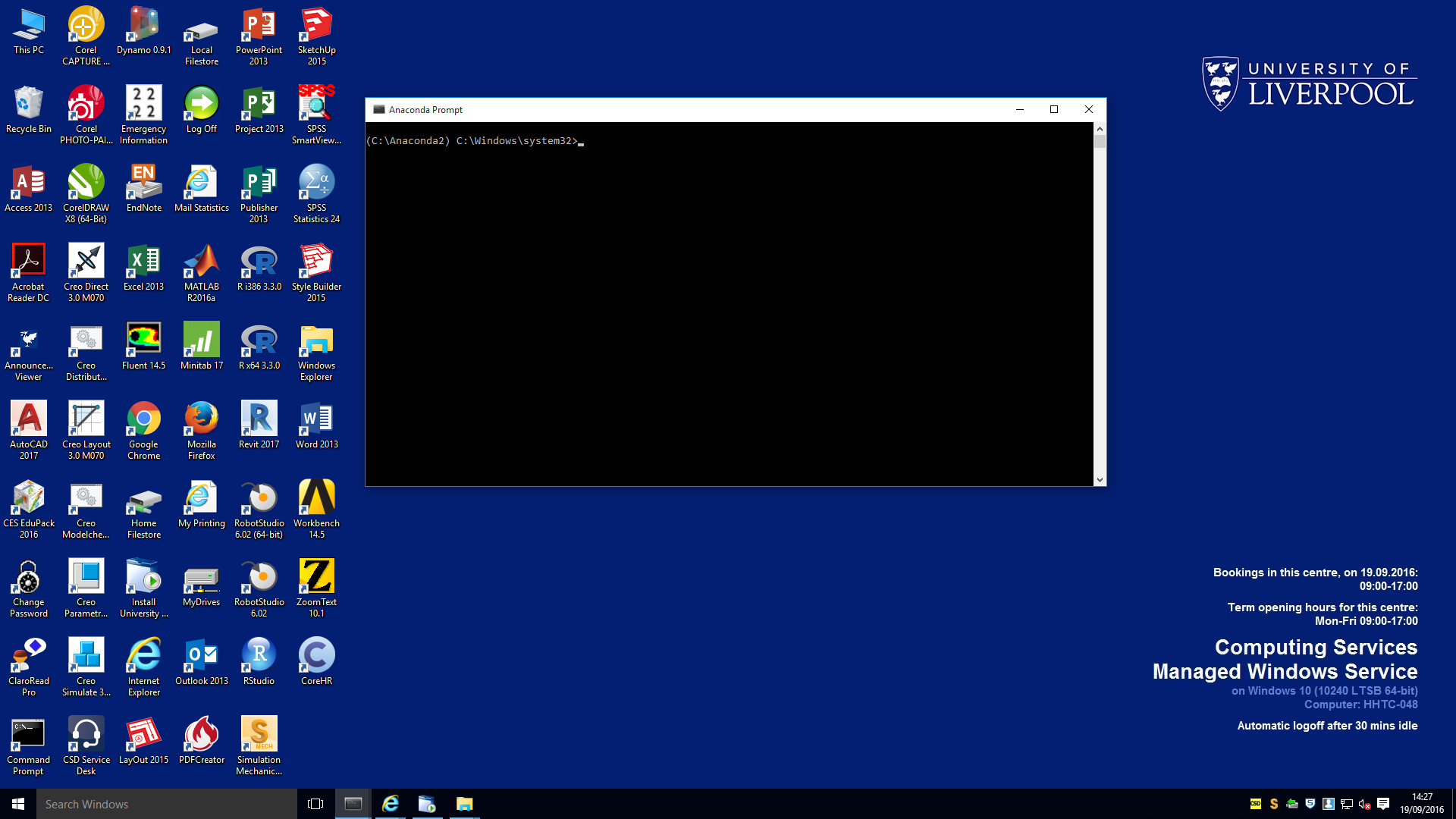
- Now you need to navigate through the computer file system (just as you would do with the Explorer window, but through commands). The first step is go to the
M:drive so everything you make is safely saved. Type the following on the prompt:
M:
which should change the C:\Windows\system32> preamble into M:\. This means you have changed to the M directory.
- Next step is activating the
gdsenvironment. For that, type the following command:
activate gds
This should set at the beginning of each prompt line the text (gds).
- At this point, you are ready to fire up the notebook! Type:
jupyter notebook
And the browser should start and open a page that looks like this:
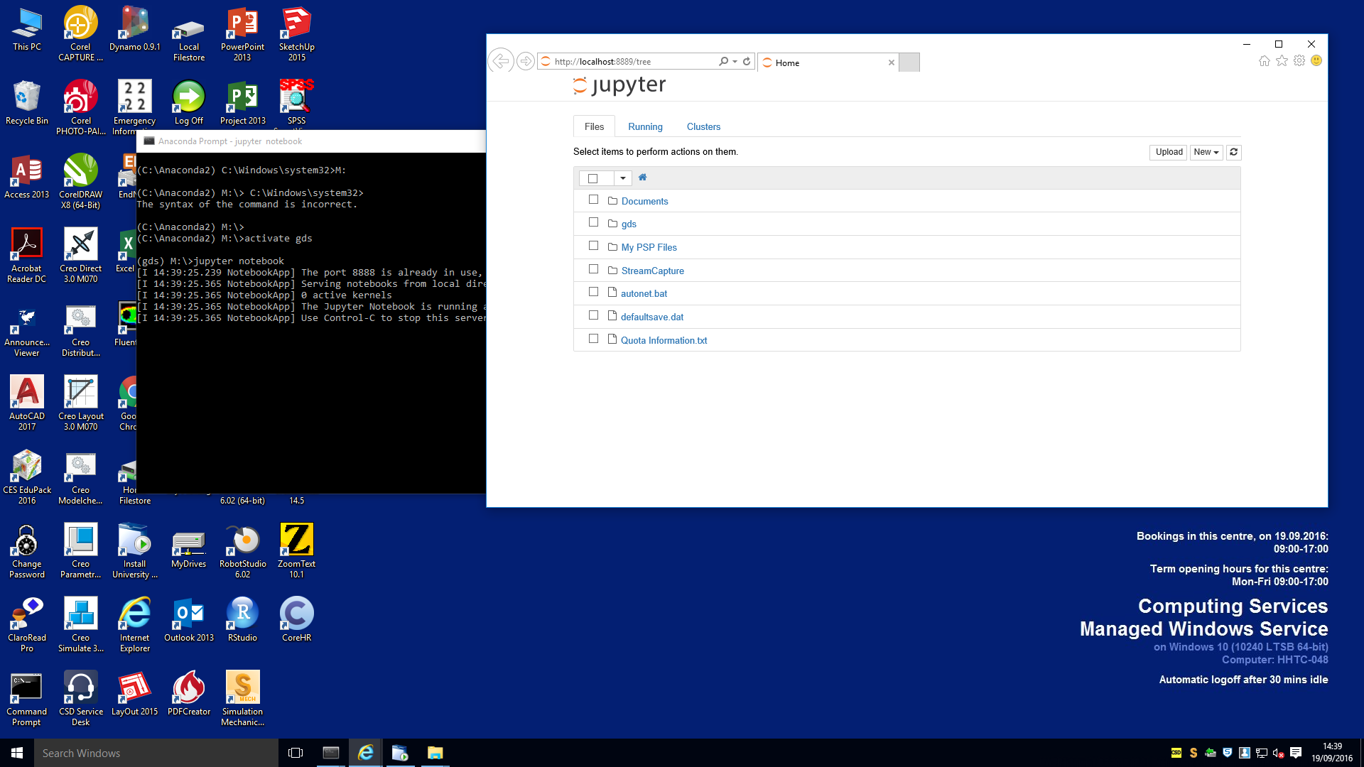
Congrats, you are good to go!!!
Download course files
Almost every file you will need for this course can be accessed through the course website:
To demonstrate how to effectively access the files needed for the computer practicals, we will use the example of the first practical. Here are the steps to follow:
- Head to the practical's page:
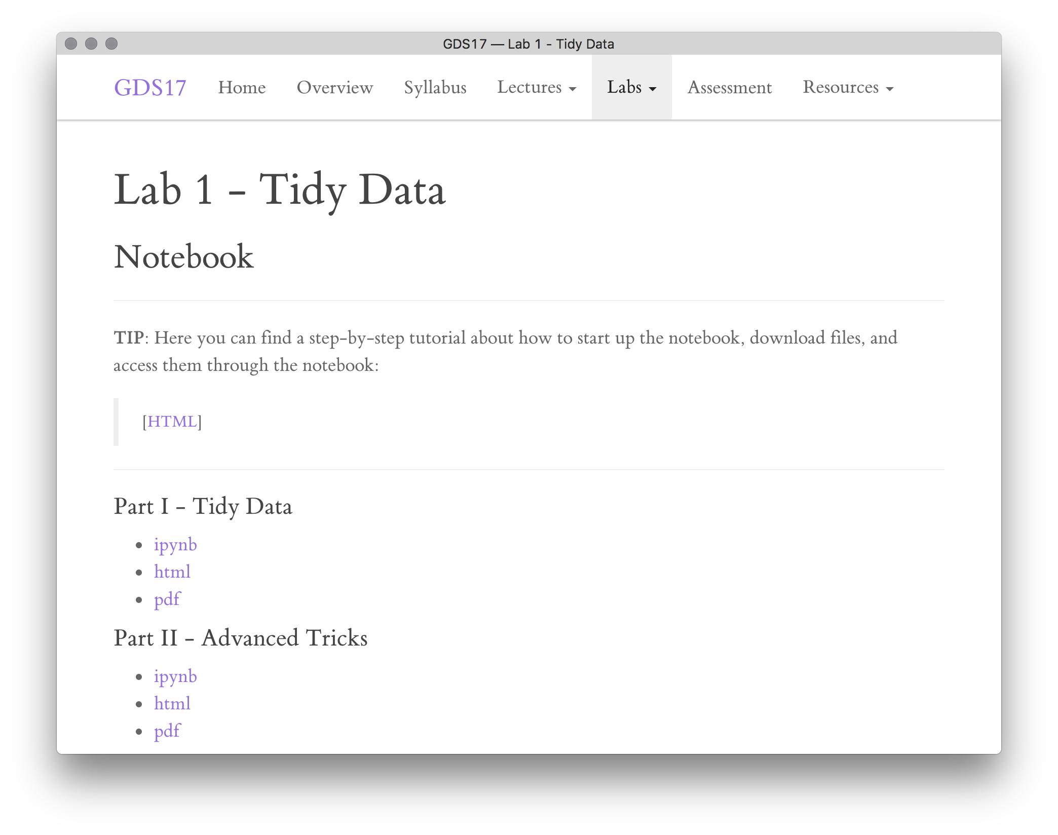
- In this case, we are interested in the first part. The file you want to download is the
ipynb, which contains the notebook. Go ahead and right-click with the mouse on top of the link (mind that if you are on a Windows machine, the menu might look slightly different, make sure to click on "Save target as").
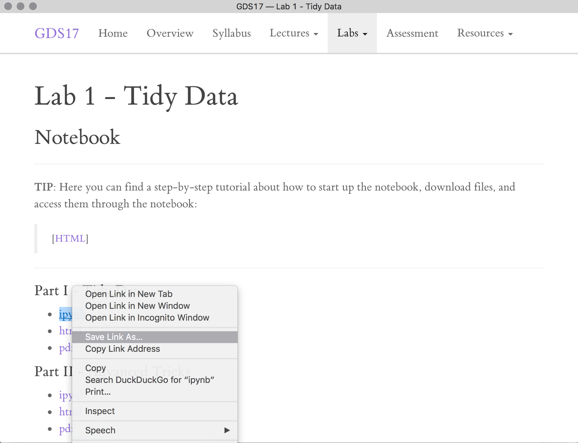
And save it somewhere WITHIN the M DRIVE. This is important for two reasons: a) you have started your Jupyter session there and b) it is the only way to ensure the file stays safely backed up and protected.
- At this point, you can go back to you Jupyter Notebook session:
And navigate within it to the folder where you have placed the notebook file.
- Click on the file and that should open a new page that looks like this:
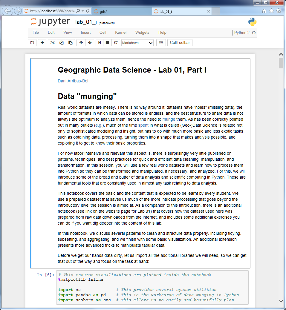
At this point, you are all set to hack some Python code!
Read files into the notebook
Finally, once you have the notebook for a practical ready, you will want to download the dataset of interest and be able to access it within the notebook. The download part is just as any other linked file from the internet; the accessing it through the notebook is a bit trickier but, once you've got around doing it once, it is always the same process.
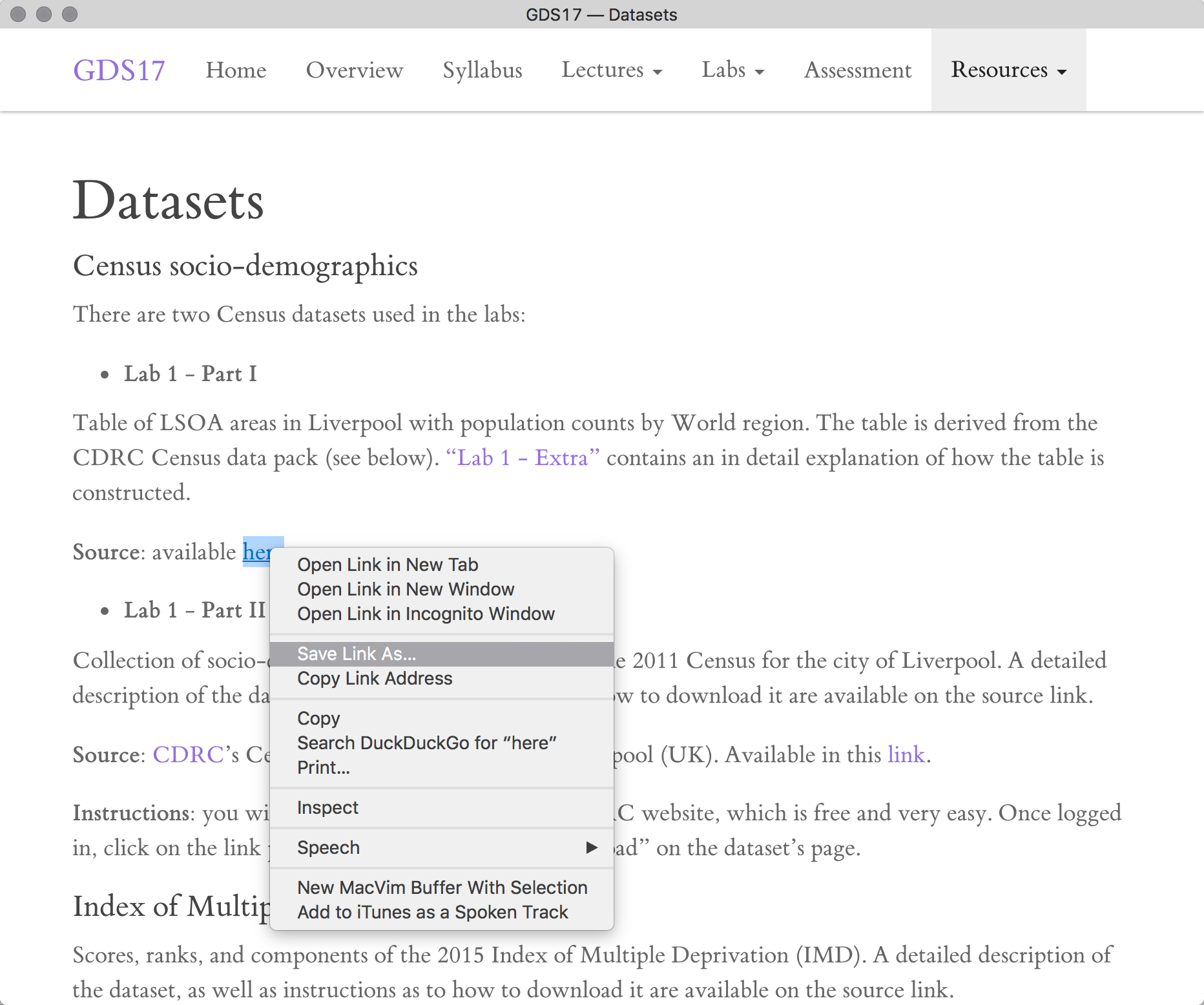
Let us use the dataset in the first lab as an example. To download it, you can access it on this link:
NOTE This is explained also in the data section of the course website.
You can download in the same way as we did the notebook before: righ-click on the link --> "Save target as..." (if on Windows, "Save link as..." otherwise). Same as before, place it somewhere within your M drive.
Now, depending on where you have saved the file, you will do one thing or another of the following:
A - If you have placed the dataset in the same folder as the notebook, all you need to do is just use the name of the file:
f = 'liv_pop.csv'
B - If you have placed the dataset in a folder within the folder where the notebook is. For example, let us assume that, within the folder where your notebook is, there is a subfolder called data. In this case, you will point to the file in this way:
f = 'data/liv_pop.csv'
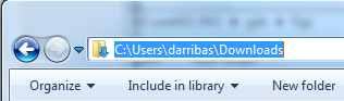
C - If you have placed the dataset in a different folder altogether. In this case, you need to obtain what is called the "full path" of the file. Let us assume you downloaded the data file into the Downloads folder. To obtain the full path, the easiest way is to open a Windows Explorer window:
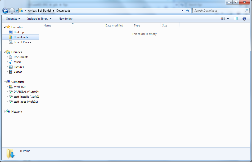
- Click on the top bar, where you would usually enter a web address if this was an internet browser. This should change it to something looking approximately like:
- Then right-click on "Desktop" and "Copy":
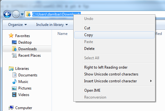
- What you have just copied is the path to the folder where the file is, and you can paste this in-lieu of the options above. However, you need to the add the name of the file (just as above):
f = "C:/Users/darribas/Downloads/liv_pop.csv"
Whichever way of the three (A, B, C) you have decided to go, you should now be ready to get on with the practical. Happy hacking!!!